
Graphing Functions with Automatic Scaling
Loading the math board and drawing, please wait…
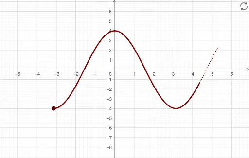
This example demonstrates how to graph a function over an open, closed, or infinite interval with automatic scaling to an appropriate window. Key math concepts include functions, intervals, automatic scaling, and function graphing. It utilizes GeoGebra commands and objects like If, Max, Min, Textfield, a1, b1, f, xr, rEnd, xl, lEnd, Mi, flEnd, Ma, MaxF, first, MinF, TB, VDf, kk, InputBox1, l, L, R, less, lessE, text1, r, less1, lessE1, InputBox2, LR, zoom, O, Graph, InputBox3, plot, Center, fi, xr1, xl1, ll, rr. Suitable for high school and above students to understand the application of function graphing and automatic scaling.
GeoGebra Commands & Parameters
If(b1 ≠ Infinity, b1, xr) → rEndIf(Defined[f(rEnd)], f(rEnd), x(Corner[2])) → frEndIf(a1 ≠ -Infinity, a1, xl) → lEndIf(Defined[y(Min[f, lEnd, rEnd])], y(Min[f, lEnd, rEnd]), y(Corner[1])) → MiIf(Defined[f(lEnd)], f(lEnd), x(Corner[1])) → flEndIf(Defined[y(Max[f, lEnd, rEnd])], y(Max[f, lEnd, rEnd]), y(Corner[4])) → MaMax({flEnd, frEnd, Ma}) → MaxFMin({Mi, flEnd, frEnd}) → MinFTextfield(a1) → InputBox1Textfield(b1) → InputBox2Textfield(f) → InputBox3If(MaxF > 10^(6) ∨ MinF < (-10^(6)), (0, 0), Intersect[Line[(lEnd, MinF), (rEnd, MaxF)], Line[(rEnd, MinF), (lEnd, MaxF)]]) → CenterIf(b1 ≟ Infinity, (2 / 3 * x(Corner[2])), b1) → xr1If(a1 ≟ -Infinity, (2 / 3 * x(Corner[1])), a1) → xl1If(a1 ≟ -Infinity, 1, 0) → llIf(b1 ≟ Infinity, 1, 0) → rrIf(MaxF > 10^(6) ∨ MinF < (-10^(6)), 1, If[abs(MaxF) < (0.45 * TB) ∧ abs(MinF) < (0.45 * TB), 1, ceil((1.3 * VDf / TB))]) → ratio
AI Drawing Prompt Reference
Draw a function graph with automatic scaling based on an interval input, showing the function's values at the endpoints and providing a suitable center point when extreme values occur. First, determine the interval endpoints, then calculate the function's values at these endpoints, find the maximum and minimum values, adjust the axes accordingly, and finally plot the function.
The prompt above was compiled from the original drawing commands and is for reference only.