
Equation Balance
Loading the math board and drawing, please wait…
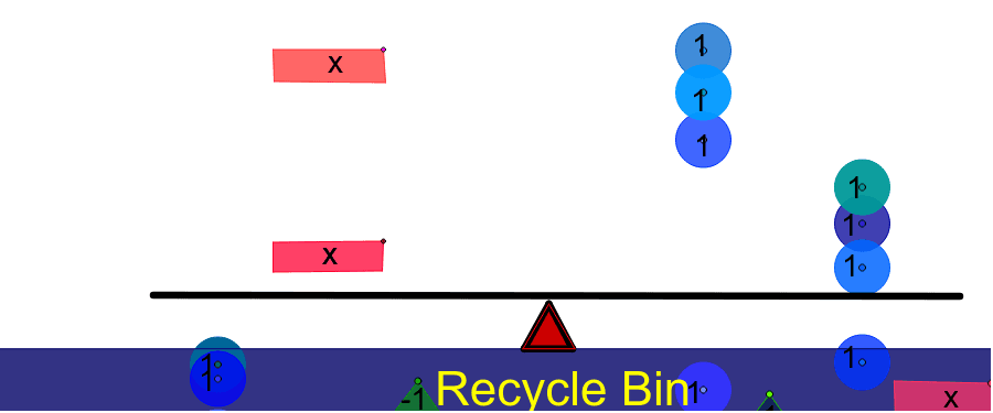
This example demonstrates the principle of equation balance. It involves core concepts of equations and functions. Using GeoGebra commands such as Segment, Point, CountIf, Circle, etc., the balance of equations can be constructed. Suitable for high school mathematics education and learning.
GeoGebra Commands & Parameters
Segment(V_2, W_2) → j_2Point(j_2) → D_3Point(j_2) → C_3Point(j_2) → Z_2CountIf(x > 0, B27:B29) → B31Segment(E, F) → cPoint(c) → TPoint(c) → SPoint(c) → RPoint(c) → QSegment(C, D) → bPoint(b) → PPoint(b) → NPoint(b) → MPoint(b) → LCountIf(x < 0, B17:B20) → B24Segment(A, B) → aPoint(a) → KPoint(a) → JPoint(a) → IPoint(a) → OCountIf(x > 0, B1:B8) → B14Segment(Q_3, R_3) → k_2Point(k_2) → T_3Point(k_2) → S_3CountIf(x > 0, A28:A29) → A32Segment(A_1, B_1) → iPoint(i) → E_1CountIf(x > 0, A13:A13) → A14Point(i) → D_1Point(i) → C_1CountIf(x > 0, A7:A8) → A10Segment(G, H) → dPoint(d) → ZPoint(d) → WPoint(d) → VPoint(d) → UCountIf(x > 0, A19:A22) → A25Segment(A_2, B_2) → a_1Circle(Q, 0.5) → eCircle(R, 0.5) → fCircle(S, 0.5) → gCircle(T, 0.5) → hCircle(I, 0.5) → kCircle(J, 0.5) → pCircle(K, 0.5) → qCircle(O, 0.5) → rCircle(U, 0.5) → sCircle(V, 0.5) → tCircle(W, 0.5) → c_1Circle(Z, 0.5) → d_1Segment(F_1, G_1) → jOrthogonalLine(C_1, i) → lOrthogonalLine(D_1, i) → mOrthogonalLine(E_1, i) → nPoint(Circle[C_1, 2.000099997500125]) → H_1Polygon(C_1, H_1, I_1, J_1) → poly1, c_2, h_1, i_1, j_1Point(Circle[D_1, 2]) → K_1Polygon(D_1, K_1, L_1, M_1) → poly2, d_2, k_1, l_1, m_1Point(a_1) → J_2Point(a_1) → K_2Point(a_1) → O_1Segment(A_3, B_3) → a_2Point(a_2) → I_3Point(a_2) → K_3Point(a_2) → O_2Segment(A_4, B_4) → a_3Point(a_3) → I_4Point(a_3) → J_4Point(a_3) → O_3Point(Circle[L, 0.8280096617793782]) → N_1Polygon(L, N_1, P_1) → poly3, p_1, l_2, n_1Point(Circle[M, 0.7161005515987262]) → Q_1Polygon(M, Q_1, R_1) → poly4, r_1, m_2, q_1Point(Circle[N, 0.6997142273814358]) → S_1Polygon(N, S_1, T_1) → poly5, t_1, n_2, s_1Point(Circle[P, 0.7211102550927978]) → U_1Polygon(P, U_1, V_1) → poly6, v_1, p_2, u_1Point(xAxis) → W_1Point(xAxis) → D_2Polygon(W_1, Z_1, C_2, D_2) → poly7, w_1, z_1, c_3, d_3Point(Circle[E_1, 2.0502987587178603]) → E_2Polygon(E_1, E_2, F_2, G_2) → poly8, e_1, e_2, f_2, g_2Point(yAxis) → H_2Point(d_3) → I_2Point(yAxis) → L_2Point(d_3) → M_2Segment(L_2, M_2) → b_1Point(d_3) → N_2Segment(L_2, N_2) → f_1Segment(M_2, N_2) → g_1Polygon(L_2, M_2, N_2) → poly9, n_3, l_3, m_3Segment(P_2, Q_2) → b_2Segment(R_2, S_2) → h_2Sum(C3:C6) → C8CountIf(x > 0, C12:C12) → C13CountIf(x > 0, D12:D12) → D13Segment(T_2, U_2) → i_2Point(Circle[Z_2, 1.8080613758656188]) → E_3Polygon(Z_2, E_3, F_3, G_3) → poly10, z_2, e_3, f_3, g_3Point(Circle[C_3, 1.697060394712511]) → H_3Polygon(C_3, H_3, J_3, L_3) → poly11, c_4, h_3, j_3, l_4Point(Circle[D_3, 1.765030632264185]) → M_3Polygon(D_3, M_3, N_3, P_3) → poly12, d_4, m_4, n_4, p_3Point(Circle[S_3, 0.7572989883260863]) → U_3Polygon(S_3, U_3, V_3) → poly13, v_3, s_3, u_3Point(Circle[T_3, 0.7697908875840829]) → W_3Polygon(T_3, W_3, Z_3) → poly14, z_3, t_3, w_3Point(f_1) → C_4Point(d_3) → D_4Polygon(C_4, D_4, 3) → poly15, q_2, r_2, s_2, E_4
AI Drawing Prompt Reference
Draw a geometric diagram illustrating equation balance, featuring two balanced segments with multiple points on each. Mark several points along each segment, and add circles with radius 0.5 at both ends of the segments to represent the balance on both sides of the equation.
The prompt above was compiled from the original drawing commands and is for reference only.