
Equation Balance Demo
Loading the math board and drawing, please wait…
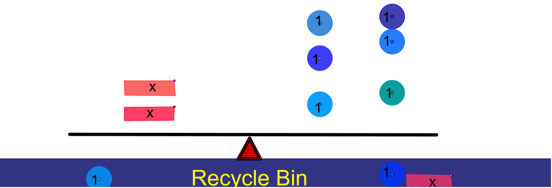
This example demonstrates interactive equation balancing through GeoGebra tools. It involves core math concepts like equation solving, inequalities, arithmetic operations, frequency distribution, continuity, LCM, and GCD. Constructed using commands like Segment, Point, CountIf, Circle, OrthogonalLine, Polygon, and Sum, it is suitable for high school and above students to explore mathematical applications of equation balancing.
GeoGebra Commands & Parameters
Segment(V_2, W_2) → j_2Point(j_2) → D_3Point(j_2) → C_3Point(j_2) → Z_2CountIf(x > 0, B27:B29) → B31Segment(E, F) → cPoint(c) → TPoint(c) → SPoint(c) → RPoint(c) → QSegment(C, D) → bPoint(b) → PPoint(b) → NPoint(b) → MPoint(b) → LCountIf(x < 0, B17:B20) → B24Segment(A, B) → aPoint(a) → KPoint(a) → JPoint(a) → IPoint(a) → OCountIf(x > 0, B1:B8) → B14Segment(Q_3, R_3) → k_2Point(k_2) → T_3Point(k_2) → S_3CountIf(x > 0, A28:A29) → A32Segment(A_1, B_1) → iPoint(i) → E_1CountIf(x > 0, A13:A13) → A14Point(i) → D_1Point(i) → C_1CountIf(x > 0, A7:A8) → A10Segment(G, H) → dPoint(d) → ZPoint(d) → WPoint(d) → VPoint(d) → UCountIf(x > 0, A19:A22) → A25Segment(A_2, B_2) → a_1Circle(Q, 0.5) → eCircle(R, 0.5) → fCircle(S, 0.5) → gCircle(T, 0.5) → hCircle(I, 0.5) → kCircle(J, 0.5) → pCircle(K, 0.5) → qCircle(O, 0.5) → rCircle(U, 0.5) → sCircle(V, 0.5) → tCircle(W, 0.5) → c_1Circle(Z, 0.5) → d_1Segment(F_1, G_1) → jOrthogonalLine(C_1, i) → lOrthogonalLine(D_1, i) → mOrthogonalLine(E_1, i) → nPoint(Circle[C_1, 2.000099997500125]) → H_1Polygon(C_1, H_1, I_1, J_1) → poly1, c_2, h_1, i_1, j_1Point(Circle[D_1, 2]) → K_1Polygon(D_1, K_1, L_1, M_1) → poly2, d_2, k_1, l_1, m_1Point(a_1) → J_2Point(a_1) → K_2Point(a_1) → O_1Segment(A_3, B_3) → a_2Point(a_2) → I_3Point(a_2) → K_3Point(a_2) → O_2Segment(A_4, B_4) → a_3Point(a_3) → I_4Point(a_3) → J_4Point(a_3) → O_3Point(Circle[L, 0.8280096617793782]) → N_1Polygon(L, N_1, P_1) → poly3, p_1, l_2, n_1Point(Circle[M, 0.7161005515987262]) → Q_1Polygon(M, Q_1, R_1) → poly4, r_1, m_2, q_1Point(Circle[N, 0.6997142273814358]) → S_1Polygon(N, S_1, T_1) → poly5, t_1, n_2, s_1Point(Circle[P, 0.7211102550927978]) → U_1Polygon(P, U_1, V_1) → poly6, v_1, p_2, u_1Point(xAxis) → W_1Point(xAxis) → D_2Polygon(W_1, Z_1, C_2, D_2) → poly7, w_1, z_1, c_3, d_3Point(Circle[E_1, 2.0502987587178603]) → E_2Polygon(E_1, E_2, F_2, G_2) → poly8, e_1, e_2, f_2, g_2Point(yAxis) → H_2Point(d_3) → I_2Point(yAxis) → L_2Point(d_3) → M_2Segment(L_2, M_2) → b_1Point(d_3) → N_2Segment(L_2, N_2) → f_1Segment(M_2, N_2) → g_1Polygon(L_2, M_2, N_2) → poly9, n_3, l_3, m_3Segment(P_2, Q_2) → b_2Segment(R_2, S_2) → h_2Sum(C3:C6) → C8CountIf(x > 0, C12:C12) → C13CountIf(x > 0, D12:D12) → D13Segment(T_2, U_2) → i_2Point(Circle[Z_2, 1.8080613758656188]) → E_3Polygon(Z_2, E_3, F_3, G_3) → poly10, z_2, e_3, f_3, g_3Point(Circle[C_3, 1.697060394712511]) → H_3Polygon(C_3, H_3, J_3, L_3) → poly11, c_4, h_3, j_3, l_4Point(Circle[D_3, 1.765030632264185]) → M_3Polygon(D_3, M_3, N_3, P_3) → poly12, d_4, m_4, n_4, p_3Point(Circle[S_3, 0.7572989883260863]) → U_3Polygon(S_3, U_3, V_3) → poly13, v_3, s_3, u_3Point(Circle[T_3, 0.7697908875840829]) → W_3Polygon(T_3, W_3, Z_3) → poly14, z_3, t_3, w_3Point(f_1) → C_4Point(d_3) → D_4Polygon(C_4, D_4, 3) → poly15, q_2, r_2, s_2, E_4
AI Drawing Prompt Reference
Draw a geometric figure for inequality balancing, including two line segments j and c, and their four points D, C, Z, T, S, R, Q, P, N, M, L. Use CountIf to count positive and negative numbers. Draw four circles centered at T, S, R, Q with a radius of 0.5.
The prompt above was compiled from the original drawing commands and is for reference only.