
Equation Balance Demonstration
Loading the math board and drawing, please wait…
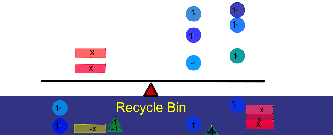
This example dynamically demonstrates the principle of equation balance, visually presenting the symmetric relationship between both sides of an equation; core math concepts include linear functions, polynomial functions, binomial distribution, and 3D vectors; construction highlights from the summary utilize commands/objects like Segment, Point, CountIf, Circle, OrthogonalLine, Polygon, Sum in GeoGebra; suitable for high school and above learners to understand equation balance and function graph transformations.
GeoGebra Commands & Parameters
Segment(V_2, W_2) → j_2Point(j_2) → D_3Point(j_2) → C_3Point(j_2) → Z_2CountIf(x > 0, B27:B29) → B31Segment(E, F) → cPoint(c) → TPoint(c) → SPoint(c) → RPoint(c) → QSegment(C, D) → bPoint(b) → PPoint(b) → NPoint(b) → MPoint(b) → LCountIf(x < 0, B17:B20) → B24Segment(A, B) → aPoint(a) → KPoint(a) → JPoint(a) → IPoint(a) → OCountIf(x > 0, B1:B8) → B14Segment(Q_3, R_3) → k_2Point(k_2) → T_3Point(k_2) → S_3CountIf(x > 0, A28:A29) → A32Segment(A_1, B_1) → iPoint(i) → E_1CountIf(x > 0, A13:A13) → A14Point(i) → D_1Point(i) → C_1CountIf(x > 0, A7:A8) → A10Segment(G, H) → dPoint(d) → ZPoint(d) → WPoint(d) → VPoint(d) → UCountIf(x > 0, A19:A22) → A25Segment(A_2, B_2) → a_1Circle(Q, 0.5) → eCircle(R, 0.5) → fCircle(S, 0.5) → gCircle(T, 0.5) → hCircle(I, 0.5) → kCircle(J, 0.5) → pCircle(K, 0.5) → qCircle(O, 0.5) → rCircle(U, 0.5) → sCircle(V, 0.5) → tCircle(W, 0.5) → c_1Circle(Z, 0.5) → d_1Segment(F_1, G_1) → jOrthogonalLine(C_1, i) → lOrthogonalLine(D_1, i) → mOrthogonalLine(E_1, i) → nPoint(Circle[C_1, 2.000099997500125]) → H_1Polygon(C_1, H_1, I_1, J_1) → poly1, c_2, h_1, i_1, j_1Point(Circle[D_1, 2]) → K_1Polygon(D_1, K_1, L_1, M_1) → poly2, d_2, k_1, l_1, m_1Point(a_1) → J_2Point(a_1) → K_2Point(a_1) → O_1Segment(A_3, B_3) → a_2Point(a_2) → I_3Point(a_2) → K_3Point(a_2) → O_2Segment(A_4, B_4) → a_3Point(a_3) → I_4Point(a_3) → J_4Point(a_3) → O_3Point(Circle[L, 0.8280096617793782]) → N_1Polygon(L, N_1, P_1) → poly3, p_1, l_2, n_1Point(Circle[M, 0.7161005515987262]) → Q_1Polygon(M, Q_1, R_1) → poly4, r_1, m_2, q_1Point(Circle[N, 0.6997142273814358]) → S_1Polygon(N, S_1, T_1) → poly5, t_1, n_2, s_1Point(Circle[P, 0.7211102550927978]) → U_1Polygon(P, U_1, V_1) → poly6, v_1, p_2, u_1Point(xAxis) → W_1Point(xAxis) → D_2Polygon(W_1, Z_1, C_2, D_2) → poly7, w_1, z_1, c_3, d_3Point(Circle[E_1, 2.0502987587178603]) → E_2Polygon(E_1, E_2, F_2, G_2) → poly8, e_1, e_2, f_2, g_2Point(yAxis) → H_2Point(d_3) → I_2Point(yAxis) → L_2Point(d_3) → M_2Segment(L_2, M_2) → b_1Point(d_3) → N_2Segment(L_2, N_2) → f_1Segment(M_2, N_2) → g_1Polygon(L_2, M_2, N_2) → poly9, n_3, l_3, m_3Segment(P_2, Q_2) → b_2Segment(R_2, S_2) → h_2Sum(C3:C6) → C8CountIf(x > 0, C12:C12) → C13CountIf(x > 0, D12:D12) → D13Segment(T_2, U_2) → i_2Point(Circle[Z_2, 1.8080613758656188]) → E_3Polygon(Z_2, E_3, F_3, G_3) → poly10, z_2, e_3, f_3, g_3Point(Circle[C_3, 1.697060394712511]) → H_3Polygon(C_3, H_3, J_3, L_3) → poly11, c_4, h_3, j_3, l_4Point(Circle[D_3, 1.765030632264185]) → M_3Polygon(D_3, M_3, N_3, P_3) → poly12, d_4, m_4, n_4, p_3Point(Circle[S_3, 0.7572989883260863]) → U_3Polygon(S_3, U_3, V_3) → poly13, v_3, s_3, u_3Point(Circle[T_3, 0.7697908875840829]) → W_3Polygon(T_3, W_3, Z_3) → poly14, z_3, t_3, w_3Point(f_1) → C_4Point(d_3) → D_4Polygon(C_4, D_4, 3) → poly15, q_2, r_2, s_2, E_4