
Energy Conservation in Undamped Spring System
Loading the math board and drawing, please wait…
In collections
MATH1052-edX
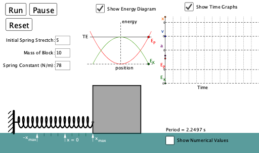
This example demonstrates the conservation of mechanical energy in an undamped spring-mass oscillator through dynamic animation, showing the periodic motion of the mass around equilibrium position where kinetic energy and elastic potential energy interchange while total energy remains constant. Core mathematical concepts include simple harmonic motion equation, differential equation solution, and energy conservation law E=½kx²+½mv²=constant. Construction highlights: using CurveCartesian to plot parametric trajectory of the oscillator, Vector and Rotate commands to construct geometric representation of the spring, Point and Segment to draw the mass and equilibrium position, Slider animation to control time parameter t演变, and Textfield to display real-time energy values. Suitable for high school physics courses teaching mechanical energy conservation, and as a physics model example for college differential equations courses.
GeoGebra Commands & Parameters
CurveCartesian((l * cur / (((2 * π) * loops))) + (p * cos(cur)) - p - ls, 2 + sin(cur), cur, 0, ((2 * π) * loops)) → curPoint(cur) → JPolygon(A, B, C, D) → poly1, a, b, c_1, dPolygon(E, F, G, H) → poly2, e, f, g, hSegment(I, J) → iPoint(xAxis) → KPoint(xAxis) → LPolygon(K, L, N, O) → poly3, k_1, l_1, n_1, o_1Vector(Q, P) → uVector(Q_1, P_1) → u_1Circle(R, (((0.5 * k) * dx_0^(2))) / 300) → cPoint(c) → SRotate(S, (360° * (abs(x(M)) / dx_0)^(2)), R) → S'Angle(S, R, S') → αCircleSector(R, S, S') → qCircleSector(R, S', S) → rPoint(r) → TPoint(r) → USegment(Z, A_1) → nSegment(B_1, C_1) → sSegment(D_1, E_1) → a_1Point(c) → J_1Point(c) → K_1Sequence(Segment[(18 + (ii * pd / 8), 21), (18 + (ii * pd / 8), 9)], ii, 5, 200, 5) → list1, {12, 12, 12, 12, 12, 12, 12, 12, 12, 12, 12, 12, 12, 12, 12, 12, 12, 12, 12, 12, 12, 12, 12, 12, 12, 12, 12, 12, 12, 12, 12, 12, 12, 12, 12, 12, 12, 12, 12, 12}Sequence(Segment[((dx_0 * iii), 0), ((dx_0 * iii), -0.5)], iii, -0.75, -0.25, 0.25) → list2, {0.5, 0.5, 0.5}Sequence(Segment[((dx_0 * iii), 0), ((dx_0 * iii), -0.5)], iii, 0.25, 0.75, 0.25) → list3, {0.5, 0.5, 0.5}Vector(Q_4, P_4) → u_4Textfield(k) → inputBox1Textfield(m) → inputBox2Textfield(dx_0) → inputBox3
AI Drawing Prompt Reference
Draw a dynamic graph showing energy conservation in a undamped spring-mass system. First, draw the geometric representation of the spring, then the mass and equilibrium position. Use a parametric curve to plot the oscillator's trajectory. Control time with a slider to display real-time kinetic and potential energy values, and draw angles and sectors on a circle to represent energy distribution.
The prompt above was compiled from the original drawing commands and is for reference only.