
Eleven Patterns of the Cube by Nolan
Loading the math board and drawing, please wait…
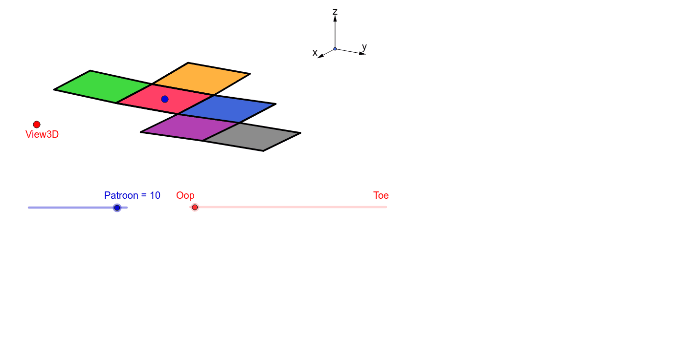
This example demonstrates the eleven possible patterns of a cube's net. It involves the concepts of solid geometry, specifically the unfolding and folding of a cube. Using commands like Vector, Translate, and Mirror, various net patterns of the cube can be constructed. Suitable for middle school and above students to learn solid geometry and spatial visualization.
GeoGebra Commands & Parameters
Vector(B_1, Z) → wVector(B_1, Y) → vVector(B_1, X) → uTranslate(A, Vector[(2 * v)]) → A'Translate(P, Vector[(2 * v)]) → P'OrthogonalLine(View3D, yAxis) → a_1OrthogonalLine(View3D, xAxis) → b_1Polygon(L, K, N, M) → poly1, l, k_1, n, mPolygon(K, P, Q, N) → poly2, k_2, p, q, n_1Polygon(L, M, S, R) → poly3, l_1, m_1, s, rPolygon(N, V, W, M) → poly4, n_2, v_1, w_1, m_2Polygon(K, T, U, L) → poly5, k_3, t, u_1, l_2Polygon(B, Q, P, A) → poly6, b_2, q_1, p_1, a_2Midpoint(R, M) → DTranslate(S, Vector[(-((2 * v)))]) → S'Segment(S, C) → eTranslate(M, Vector[((-2) * v)]) → M'Segment(M, E) → fSegment(E, C) → hTranslate(N, Vector[((-2) * v)]) → N'Translate(Q, Vector[((-2) * v)]) → Q'_1Segment(Q, F) → iSegment(N, G) → jSegment(G, F) → d_1Translate(Q, Vector[((-2) * v)]) → Q'_2Translate(B, Vector[((-2) * v)]) → B'_1Segment(B, I) → e_1Segment(I, H) → f_1Segment(H, Q) → g_1Translate(K, Vector[(2 * v)]) → K'Translate(P, Vector[(2 * v)]) → P'_1Segment(P, J) → h_1Segment(J, A_1) → i_1Segment(A_1, K) → j_1Segment(B, H_1) → s_1Segment(H_1, C_1) → cSegment(C_1, A) → r_1Midpoint(N, P) → D_1Midpoint(k_1) → F_1Segment(A, G_1) → t_1Segment(G_1, I_1) → c_2Segment(I_1, P) → d_2Segment(J, K_1) → f_2Segment(P, L_1) → e_2Segment(L_1, K_1) → g_2Segment(M, W) → h_2Mirror(L_1, F_1) → O_1Mirror(K_1, F_1) → P_1Segment(M, M_1) → i_2Segment(N_1, J_1) → j_2Segment(J_1, M_1) → p_2Polygon(M, E, C, S) → poly7, q_2, r_2, s_2, t_2Polygon(Q, N, G, F) → poly8, q_3, n_3, g_3, f_3Polygon(B, Q, H, I) → poly9, b_3, q_4, h_3, i_3Polygon(J, A_1, K, P) → poly10, j_3, a_3, k_4, p_3Polygon(C_1, A, B, H_1) → poly11, c_3, a_4, b_4, h_4Polygon(G_1, I_1, P, A) → poly12, g_4, i_4, p_4, a_5Polygon(K_1, J, P, L_1) → poly13, k_5, j_4, p_5, l_3Polygon(M, M_1, J_1, N_1) → poly14, m_3, m_4, j_5, n_4
AI Drawing Prompt Reference
Draw the eleven possible nets of a cube by first defining three orthogonal vectors, then translating a base square along these vectors to create adjacent squares, using orthogonal lines to set the drawing plane, constructing six square faces, marking the midpoints of edges, translating vertices back along the vectors to form corresponding points, connecting segments to outline each net, and finally mirroring points across midpoints to complete the remaining two net patterns.
The prompt above was compiled from the original drawing commands and is for reference only.