
Dynamic Graphs of Linear and Quadratic Inequalities with Sliders
Loading the math board and drawing, please wait…
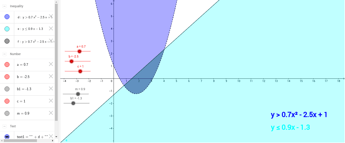
This GeoGebra example demonstrates the graphs of linear and quadratic inequalities in the Cartesian coordinate plane, allowing users to adjust coefficients and constants in real time using sliders to observe how solution regions change shape and position. Core mathematical concepts include linear inequalities, quadratic inequalities, function graphs, solution sets, half-planes, regions inside and outside parabolas, inequality direction, and boundary line styles such as solid versus dashed lines. Construction details: GeoGebra objects b1, m, a, b, c, d, e control line slope, intercept, and quadratic coefficients; text1 and text2 display dynamic inequality expressions; f represents the function graph; and slider-driven parameter animation links all elements together. Suitable for middle school and high school mathematics instruction, classroom demonstrations, independent inquiry, and visualization practice of inequality solution sets.
GeoGebra Commands & Parameters
Numeric b1(-1.3)Numeric m(0.9)Numeric a(0.7)Numeric b(-2.5)Numeric c(1.0)y > a * x^(2) + b * x + cy ≤ m * x + b1d(x, y) ∧ e(x, y)
AI Drawing Prompt Reference
Draw a Cartesian coordinate plane with two inequality solution regions. One region is for a linear inequality y ≤ mx + b, bounded by a solid straight line with adjustable slope and intercept. The other is for a quadratic inequality y > ax² + bx + c, bounded by a dashed upward-opening parabola with adjustable coefficients. Shade the intersection of the two regions distinctly. Include text labels showing the current inequality expressions. Use sliders to adjust all coefficients dynamically, allowing the regions to change shape and position in real time.
The prompt above was compiled from the original drawing commands and is for reference only.