
Dynamic Derivative Loupe II
Loading the math board and drawing, please wait…
In collections
ICME 13, TSG 16: A visual approach to calculus
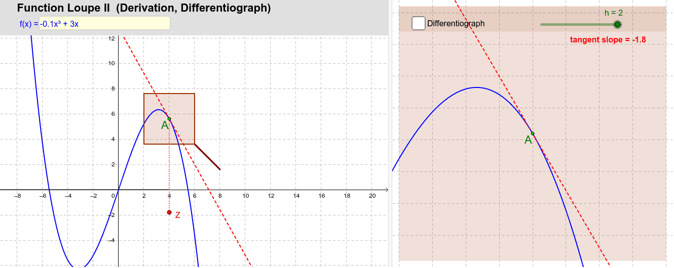
This example demonstrates the functionality of a dynamic derivative loupe, using dynamic derivative plots to help understand the concept of derivatives. Key mathematical concepts include derivatives, functions, and trigonometric functions. It utilizes multiple GeoGebra commands such as text fields, points, polygons, midpoints, segments, if conditions, tangents, slopes, and loci. Suitable for high school and above students or teachers, it aids in a deeper understanding of the local properties of functions.
GeoGebra Commands & Parameters
Textfield(f) → Textfeld1Point(f) → APolygon(A + ((-h), (-h)), A + (h, (-h)), A + (h, h), A + ((-h), h)) → Lupe, i, j, k, lMidpoint(A_l, Al) → BMidpoint(A, Ar) → CSegment(A_l, Al) → bSegment(A + (h, (-h)), A + (2 * (h, (-h)))) → griff1Segment(A + (min, (-min)), A + (2 * (min, (-min)))) → griff2If(h > min, griff1, griff2) → griffPolygon(F, G, D, E) → Vieleck4, f_2, g_2, d_2, e_2Tangent(A, f) → tangenteSlope(tangente) → steigungLocus(Z, A) → Ortslinie1Ray(H, I) → aPoint(a) → XTangent(A1, f) → tang1Slope(tang1) → stLocus(J, X) → Ortslinie2Segment(A, Z) → c