
Dynamic Demonstration of the Centre of Mass of a Lamina Between Two Curves
Loading the math board and drawing, please wait…
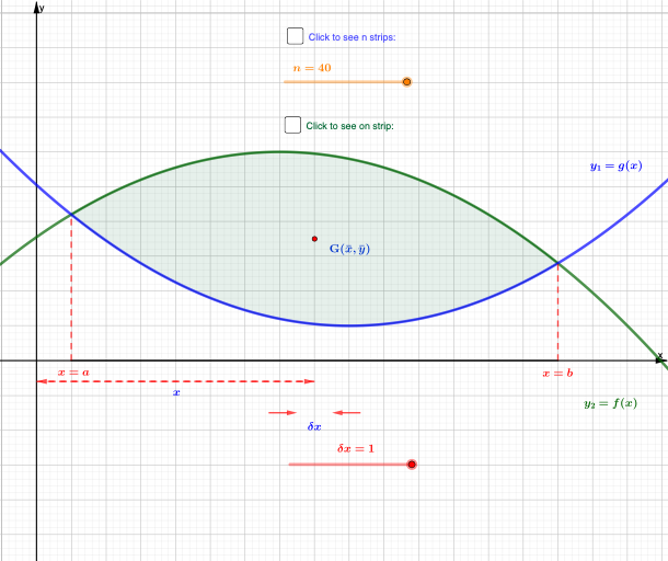
This GeoGebra example dynamically demonstrates the centre of mass of a thin lamina bounded by two curves. The core mathematical concept is the calculation of the centroid (centre of mass) using definite integrals, involving area and first moments. Construction highlights include: Intersect to find curve intersections, IntegralBetween to compute the area, Integral for moments, Point and Midpoint to construct key points, Vector to represent the centroid vector, Segment and Polygon for visual aids, Sequence to create partition strips, and Slider for parameter variation. Suitable for high school or early university calculus and physics courses, it helps students intuitively grasp the geometric meaning of the centroid formula.
GeoGebra Commands & Parameters
Intersect(f, g) → A, B, C_{1}, D_{1}Integral((x * h(x)), x(A), x(B)) → bIntegralBetween(f, g, x(A), x(B)) → aPoint(xAxis) → CSegment(C, A) → iPoint(xAxis) → DSegment(D, B) → jSegment(C, D) → kSegment(D, C) → lSequence((1 + ((k - 1) * d), g(1 + ((k - 1) * d))), k, 1, n) → l1, {(1, 4.2), (1.35, 3.9261250000000008), (1.7, 3.6645000000000003), (2.05, 3.415125), (2.4, 3.178), (2.75, 2.953125), (3.0999999999999996, 2.7405), (3.4499999999999997, 2.5401250000000006), (3.8, 2.3520000000000003), (4.15, 2.176125), (4.5, 2.0125), (4.85, 1.8611250000000004), (5.199999999999999, 1.7220000000000004), (5.55, 1.5951250000000001), (5.8999999999999995, 1.4805000000000001), (6.25, 1.378125), (6.6, 1.288), (6.949999999999999, 1.2101250000000001), (7.3, 1.1445), (7.6499999999999995, 1.0911250000000001), (8, 1.05), (8.35, 1.021125), (8.7, 1.0045), (9.049999999999999, 1.000125), (9.399999999999999, 1.008), (9.75, 1.028125), (10.1, 1.0605), (10.45, 1.105125), (10.799999999999999, 1.162), (11.149999999999999, 1.2311249999999998), (11.5, 1.3125), (11.85, 1.4061249999999998), (12.2, 1.5119999999999998), (12.549999999999999, 1.6301249999999996), (12.899999999999999, 1.7604999999999995), (13.25, 1.9031250000000002), (13.6, 2.058), (13.95, 2.225125), (14.299999999999999, 2.4044999999999996), (14.649999999999999, 2.5961249999999993)}Sequence((1 + ((k - 1) * d), g(x(l1(2)) + ((k - 1) * d))), k, 1, n) → l4, {(1, 3.9261250000000008), (1.35, 3.6645000000000003), (1.7, 3.415125), (2.05, 3.178), (2.4, 2.953125), (2.75, 2.7405), (3.0999999999999996, 2.5401250000000006), (3.4499999999999997, 2.3520000000000003), (3.8, 2.176125), (4.15, 2.0125), (4.5, 1.8611250000000004), (4.85, 1.7220000000000004), (5.199999999999999, 1.5951250000000003), (5.55, 1.4805), (5.8999999999999995, 1.378125), (6.25, 1.288), (6.6, 1.2101250000000001), (6.949999999999999, 1.1445000000000003), (7.3, 1.091125), (7.6499999999999995, 1.05), (8, 1.021125), (8.35, 1.0045), (8.7, 1.000125), (9.049999999999999, 1.008), (9.399999999999999, 1.028125), (9.75, 1.0605), (10.1, 1.105125), (10.45, 1.162), (10.799999999999999, 1.2311249999999998), (11.149999999999999, 1.3124999999999996), (11.5, 1.4061249999999998), (11.85, 1.5119999999999998), (12.2, 1.6301249999999996), (12.549999999999999, 1.7604999999999995), (12.899999999999999, 1.9031249999999993), (13.25, 2.058), (13.6, 2.225125), (13.95, 2.4044999999999996), (14.299999999999999, 2.5961249999999993), (14.649999999999999, 2.799999999999999)}Sequence((1 + ((k - 1) * d), f(x(l1(2)) + ((k - 1) * d))), k, 1, n) → l2, {(1, 4.403874999999999), (1.35, 4.5954999999999995), (1.7, 4.774875), (2.05, 4.942), (2.4, 5.096875), (2.75, 5.2395), (3.0999999999999996, 5.3698749999999995), (3.4499999999999997, 5.4879999999999995), (3.8, 5.593875), (4.15, 5.6875), (4.5, 5.7688749999999995), (4.85, 5.838), (5.199999999999999, 5.894875), (5.55, 5.9395), (5.8999999999999995, 5.971875), (6.25, 5.992), (6.6, 5.999875), (6.949999999999999, 5.9955), (7.3, 5.978875), (7.6499999999999995, 5.95), (8, 5.908875), (8.35, 5.8555), (8.7, 5.789875), (9.049999999999999, 5.712000000000001), (9.399999999999999, 5.621875), (9.75, 5.5195), (10.1, 5.4048750000000005), (10.45, 5.2780000000000005), (10.799999999999999, 5.1388750000000005), (11.149999999999999, 4.987500000000001), (11.5, 4.823875), (11.85, 4.648000000000001), (12.2, 4.459875), (12.549999999999999, 4.259500000000001), (12.899999999999999, 4.046875000000001), (13.25, 3.822), (13.6, 3.5848750000000003), (13.95, 3.3355000000000006), (14.299999999999999, 3.073875000000001), (14.649999999999999, 2.800000000000001)}Sequence((x(l1(2)) + ((k - 1) * d), f(x(l1(2)) + ((k - 1) * d))), k, 1, n) → l3, {(1.35, 4.403874999999999), (1.7000000000000002, 4.5954999999999995), (2.05, 4.774875), (2.4, 4.942), (2.75, 5.096875), (3.1, 5.2395), (3.4499999999999997, 5.3698749999999995), (3.8, 5.4879999999999995), (4.15, 5.593875), (4.5, 5.6875), (4.85, 5.7688749999999995), (5.199999999999999, 5.838), (5.549999999999999, 5.894875), (5.9, 5.9395), (6.25, 5.971875), (6.6, 5.992), (6.949999999999999, 5.999875), (7.299999999999999, 5.9955), (7.65, 5.978875), (8, 5.95), (8.35, 5.908875), (8.7, 5.8555), (9.049999999999999, 5.789875), (9.399999999999999, 5.712000000000001), (9.749999999999998, 5.621875), (10.1, 5.5195), (10.45, 5.4048750000000005), (10.799999999999999, 5.2780000000000005), (11.149999999999999, 5.1388750000000005), (11.499999999999998, 4.987500000000001), (11.85, 4.823875), (12.2, 4.648000000000001), (12.549999999999999, 4.459875), (12.899999999999999, 4.259500000000001), (13.249999999999998, 4.046875000000001), (13.6, 3.822), (13.95, 3.5848750000000003), (14.299999999999999, 3.3355000000000006), (14.649999999999999, 3.073875000000001), (14.999999999999998, 2.800000000000001)}Polygon(E, F, I, H) → q1, e, f_1, i_1, h_1Vector(J, K) → uVector(K, J) → vMidpoint(J, K) → LVector(M, N) → wVector(N, M) → cMidpoint(M, N) → OVector(Q, P) → mVector(S, R) → qSequence(Polygon[(1 + ((k - 1) * d), f(x(l1(2)) + ((k - 1) * d))), (x(l1(2)) + ((k - 1) * d), f(x(l1(2)) + ((k - 1) * d))), (x(l1(2)) + ((k - 1) * d), g(x(l1(2)) + ((k - 1) * d))), (x(l1(1)) + ((k - 1) * d), g(x(l1(2)) + ((k - 1) * d)))], k, 1, n - 1) → l5, {0.16721249999999888, 0.32585, 0.47591249999999974, 0.6173999999999991, 0.7503124999999988, 0.874649999999999, 0.9904124999999997, 1.0975999999999981, 1.1962125000000006, 1.28625, 1.3677124999999961, 1.440599999999998, 1.5049125000000014, 1.5606500000000025, 1.6078125000000085, 1.6463999999999945, 1.6764124999999996, 1.697849999999999, 1.7107124999999996, 1.7150000000000034, 1.7107124999999996, 1.697849999999999, 1.6764124999999943, 1.6463999999999999, 1.6078125000000014, 1.5606499999999954, 1.5049124999999997, 1.4405999999999963, 1.3677124999999997, 1.2862500000000026, 1.196212499999998, 1.0976, 0.990412500000005, 0.8746500000000008, 0.7503125000000033, 0.6173999999999964, 0.47591249999999974, 0.32584999999999553, 0.167212499999998}
AI Drawing Prompt Reference
Draw two function curves that intersect within an interval, forming an enclosed region between them. Divide this region into several vertical strips along the horizontal direction, representing each strip as a polygon. Select two points on the x-axis and draw perpendicular lines to the intersection points of the two curves, creating a reference rectangle. Calculate the area between the curves and the first moment about the y-axis to determine the centroid location, then use vectors pointing from the region boundary to the centroid to visually display its position. A slider can adjust the number of strips to observe how the centroid approaches its exact value as the division becomes finer.
The prompt above was compiled from the original drawing commands and is for reference only.