
Dynamic Demonstration of Area Concept: Polygon Decomposition and Reassembly
Loading the math board and drawing, please wait…
In collections
AREA
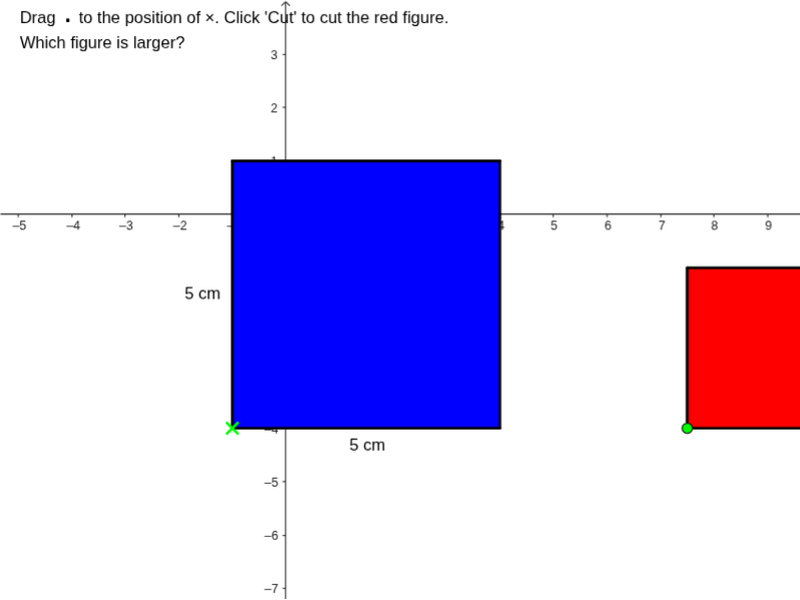
① This example dynamically demonstrates the concept of area by cutting, translating, and reassembling polygons (such as rectangles and trapezoids) to show that area remains invariant under such transformations, emphasizing that area measures the interior region of a shape regardless of its form. ② Core mathematical concepts include area, perimeter, polygons, rectangles, squares, trapezoids, definite integral (as an extension of area), median line, random variables, and linear programming (possibly for area optimization), but the main focus is on additivity and conservation of area. ③ Construction highlights: From the construction summary, the example uses GeoGebra commands such as Polygon to create multiple polygons (poly1 to poly8), If for conditional control of the cutting process, and Midpoint to generate midpoints for auxiliary divisions. It involves multiple points (A, B, C, D, E) and segments (a, h, i, j, k, l, m, n, p, q, r, s, t, etc.) to build cutting paths. Objects labeled '剪開第一次', '剪開第二次', '剪開第三次' indicate a step-by-step animation showing area conservation. ④ Suitable for upper elementary to middle school students learning area concepts, and also useful for high school review of geometry and integral connections. It serves as a dynamic teaching aid for classroom demonstrations or student self-exploration of area additivity.
GeoGebra Commands & Parameters
Polygon(A, (x(A) + 5, y(A)), (x(A) + 5, y(A) + 3), (x(A), y(A) + 3)) → poly3, a_1, h, i, jPolygon(C, (x(C) + 3, y(C)), (x(C) + 3, y(C) + 3), (x(C), y(C) + 3)) → poly4, c_1, k, l, mPolygon((x(A), y(A) + 3), (x(A) + 3, y(A) + 3), (x(A) + 3, y(A) + 5), (x(A), y(A) + 5)) → poly5, n, p, q, rPolygon(D, (x(D) + 3, y(D)), (x(D) + 3, y(D) + 1), (x(D), y(D) + 1)) → poly6, d_1, s, t, e_1Polygon((x(A) + 3, y(A) + 3), (x(A) + 5, y(A) + 3), (x(A) + 5, y(A) + 4), (x(A) + 3, y(A) + 4)) → poly7, f_1, g_1, h_1, i_1Polygon(E, (x(E) + 1, y(E)), (x(E) + 1, y(E) + 1), (x(E), y(E) + 1)) → poly8, e_2, j_1, k_1, l_1Polygon(A, (x(A) + 5, y(A)), (x(A) + 5, y(A) + 5), (x(A), y(A) + 5)) → poly1, a, b, c, dPolygon(B, (x(B) + 8, y(B)), (x(B) + 8, y(B) + 3), (x(B), y(B) + 3)) → poly2, b_1, e, f, gPolygon((7.5, -4), (15.5, -4), (15.5, -1), (7.5, -1)) → poly9, m_1, n_1, p_1, q_1If(E ≟ H, true, false) → 返回原位Polygon(A1, (x(A1) + 5, y(A1)), (x(A1) + 5, y(A1) + 3), (x(A1), y(A1) + 3)) → poly10, a1, r_1, s_1, t_1Polygon(A2, (x(A2) + 3, y(A2)), (x(A2) + 3, y(A2) + 2), (x(A2), y(A2) + 2)) → poly11, a2, a_2, b_2, c_2Polygon(A3, (x(A3) + 2, y(A3)), (x(A3) + 2, y(A3) + 1), (x(A3), y(A3) + 1)) → poly12, a3, d_2, f_2, g_2Polygon(A4, (x(A4) + 1, y(A4)), (x(A4) + 1, y(A4) + 1), (x(A4), y(A4) + 1)) → poly13, a4, h_2, i_2, j_2Midpoint(a) → JMidpoint(m_1) → KMidpoint(n_1) → LMidpoint(d) → I
AI Drawing Prompt Reference
Create a dynamic diagram demonstrating area conservation: start with a large rectangle, then divide it internally into smaller rectangles and trapezoids using line segments. These pieces can be translated and reassembled while the total area remains unchanged. Include several independent rectangles and trapezoids, with midpoints used for auxiliary divisions. Use sliders to control the cutting and moving steps. The layout has two parts: the upper part shows the original shapes, and the lower part shows the reassembled shapes, illustrating that the area stays the same. All polygons have solid borders and may be filled with different colors for distinction.
The prompt above was compiled from the original drawing commands and is for reference only.