
Dependent Difference Tests: Writing Conclusions
Loading the math board and drawing, please wait…
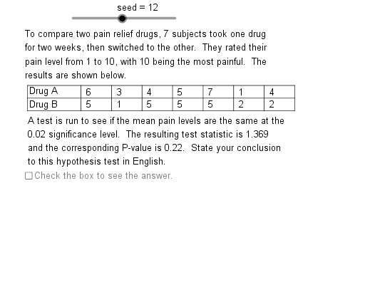
This example demonstrates how to perform dependent difference tests and write conclusions. Key mathematical concepts include hypothesis testing and statistics. Using GeoGebra commands such as Sequence, Element, Length, Mean, etc., a series of data sets are constructed and analyzed.
GeoGebra Commands & Parameters
Sequence(Mod[5 + (13 * k), 29] + 20, k, 1, 24) → OpSqElement(OpSq, seed) → Nmb1Element(CnfSq, Chc2) → ConfElement(DtASq, Chc1) → DtAElement(DtBSq, Chc1) → DtBLength(DtA) → SizeSequence(Element[DtA, k] - Element[DtB, k], k, 1, Size) → DffSqMean(DffSq) → XbarSampleSD(DffSq) → StDvIf(PVl < α, 1, 0) → CmprIf(Cmpr ≟ 1, "rejected", "kept") → DcsnIf(Cmpr ≟ 1, "is", "is not") → ConStmtIf(PVl < α, " less than ", If[PVl > α, " more than ", " equal to"]) → IneqSqnIf(TstSt < 0, "1E99", TstSt) → UBTxIf(TstSt < 0, "-1E99", TstSt) → LBTxIf(PVl < 5.0E-4, 5.0E-4, PVl) → SmPVIf(PVl < 5.0E-4, "is less than", "is about") → PVIEElement(LbASq, Chc1) → LbAElement(LbBSq, Chc1) → LbBSequence(Segment[(0.6, TbTp - (0.5 * k)), (2.7 + (CW * Size), TbTp - (0.5 * k))], k, 0, 2) → HzLnSequence(Text[Element[DtA, k], (1.7 + (CW * k), TbTp - 0.38)], k, 1, Size) → DtATxSequence(Text[Element[DtB, k], (1.7 + (CW * k), TbTp - 0.88)], k, 1, Size) → DtBTxSequence(Segment[(2.7 + (1.2 * k), TbTp), (2.7 + (1.2 * k), TbTp - 1)], k, 0, Size) → VrLnSegment((0.6, TbTp), (0.6, TbTp - 1)) → tblf
AI Drawing Prompt Reference
Create a statistical chart showing data sequences and difference analysis. Generate two sequences of data with different colors, calculate their differences, and plot the mean and standard deviation of the differences. Label the conclusion based on hypothesis testing, such as rejecting or keeping the null hypothesis. Add text labels for data points and conclusions, along with horizontal and vertical line segments as guides.
The prompt above was compiled from the original drawing commands and is for reference only.