
Demonstration of Spiral Infinity
Loading the math board and drawing, please wait…
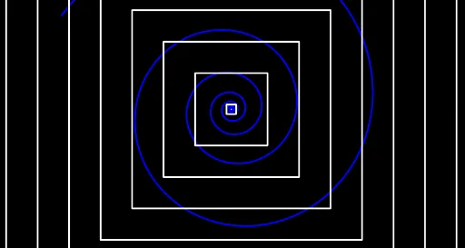
This example demonstrates the infinite nature of a spiral in time and space. It involves core mathematical concepts such as parametric curves, coordinate geometry, and geometric transformations. Key GeoGebra commands and objects used in the construction include CurveCartesian, Ray, Angle, Circle, Intersect, Segment, Line, Mirror, Polygon, Dilate, and Sequence. It is suitable for high school and above students to understand the application of parametric curves and geometric transformations.
GeoGebra Commands & Parameters
CurveCartesian(((r_0 / a^(3.141592653589793) * a^(t)) * cos(t)), ((r_0 / a^(3.141592653589793) * a^(t)) * sin(t)), t, -31.41593, 12.56637) → gCurveCartesian(((r_0 / a^((3 * 3.141592653589793 / 2)) * a^(t)) * cos(t)), ((r_0 / a^((3 * 3.141592653589793 / 2)) * a^(t)) * sin(t)), t, -31.41593, 12.56637) → hCurveCartesian((((r_0 * a^(3.141592653589793 / 2)) * a^(t)) * cos(t)), (((r_0 * a^(3.141592653589793 / 2)) * a^(t)) * sin(t)), t, -31.41593, 12.56637) → iCurveCartesian(((r_0 / a^(3.141592653589793 / 2) * a^(t)) * cos(t)), ((r_0 / a^(3.141592653589793 / 2) * a^(t)) * sin(t)), t, -31.41593, 12.56637) → fRay(B, A) → cAngle(xAxis, c) → βCurveCartesian(((r_0 * a^(t)) * cos(t)), ((r_0 * a^(t)) * sin(t)), t, -31.41593, 6.283185307179586) → a_1Circle(B, 5.5) → dIntersect(d, c, 1) → ESegment(B, E) → jLine(H, xAxis) → kLine(J, yAxis) → lMirror(l, yAxis) → l'Mirror(k, xAxis) → k'Intersect(k, l') → KIntersect(k, l) → LIntersect(k', l) → MIntersect(l', k') → NPolygon(K, L, M, N) → q1, k_1, l_1, m, nPolygon(K, L, M, N) → q2, k_2, l_2, m_1, n_1Dilate(K, 2, B) → K'Dilate(L, 2, B) → L'Dilate(M, 2, B) → M'Dilate(N, 2, B) → N'Polygon(K', L', M', N') → q2', p, q, m', n'CurveCartesian(((r_0 * a^(t + α)) * cos(t + α)), ((r_0 * a^(t + α)) * sin(t + α)), t, -31.41593, (2 * π) + α) → oLine(B, N) → rLine(B, M) → sSequence(Polygon[Dilate[K, i, B], Dilate[L, i, B], Dilate[M, i, B], Dilate[N, i, B]], i, -1, 3, 0.25) → l1Sequence((x(B) + (n * λ) + Mod[(v_p * v), λ], 0), n, 0, Ni) → l2Sequence((0, x(B) + (n * λ) + Mod[(v_p * v), λ]), n, 0, Ni) → l3Sequence(Line[Element[l2, i], yAxis], i, 1, Length[l2]) → l5Sequence(Line[Element[l3, i], xAxis], i, 1, Length[l3]) → l4Sequence(Intersect[Element[l4, i], Element[l5, i]], i, 1, Length[l5]) → l6Mirror(l6, yAxis) → l6'Sequence(Polygon[Element[l6, i], Element[l6', i], 4], i, 1, Length[l6]) → l7CurveCartesian(((r_0 * a^(t + α)) * cos(t)), ((r_0 * a^(t + α)) * sin(t)), t, -36.41593, (2 * π) + α) → b
AI Drawing Prompt Reference
Draw a logarithmic spiral centered at the origin, extending from negative to positive angles, with several phase-shifted spiral branches. Place a point near the center, draw a ray from it intersecting the spiral, and construct a circle centered at that point. Create horizontal and vertical auxiliary lines through the point, use symmetry and reflection to form a rectangular grid, then scale the grid vertices to produce nested rectangles. Finally, generate multiple sets of parallel lines along the spiral direction, intersecting the grid to create a dynamic spiral extension effect.
The prompt above was compiled from the original drawing commands and is for reference only.