
Demonstrating the Range of Inverse Trigonometric Functions
Loading the math board and drawing, please wait…
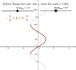
This example illustrates inverse trigonometric functions and why their output ranges are limited. It covers the domains, ranges, and symmetries of functions like sine, cosine, and their inverses. Constructed using GeoGebra commands such as SelectedElement, Mirror, and SurdText. Suitable for high school mathematics education to understand the properties and range limitations of inverse trigonometric functions.
GeoGebra Commands & Parameters
SelectedElement(fcns) → fMirror(f, g) → f_1Mirror(flim, g) → flim_1SurdText(Range_{max}, {π}) → r_maxSurdText(Range_{min}, {π}) → r_min
AI Drawing Prompt Reference
Draw a graph illustrating the range limitations of inverse trigonometric functions, including sine and cosine functions along with their inverses, show symmetry through mirror operations, and label the maximum and minimum value ranges of the inverse functions using π units, with the construction sequence being first to plot the base functions, then perform mirror operations, and finally annotate the key numerical ranges.
The prompt above was compiled from the original drawing commands and is for reference only.