
Curvy Slide: Square Cross Sections with Polynomial Regression
Loading the math board and drawing, please wait…
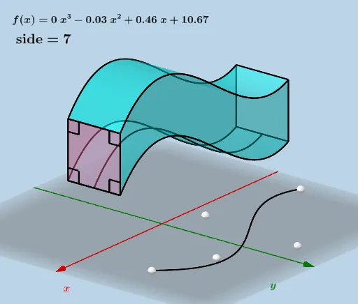
This GeoGebra example demonstrates a 3D solid sliding along a curved path, featuring square cross sections that can be dynamically adjusted via a polynomial regression curve. It visualizes the interplay between solid geometry and calculus, particularly the method of cross sections for approximating volumes. Core mathematical concepts include polynomial fitting, parametric curves, 3D transformations (translation and rotation), and Riemann sums (upper and lower sums) as a limit process. The construction uses commands such as FitPoly to generate the regression curve from points, PointIn, Point, Plane, Segment, and Surface to build the 3D framework, Rotate, Mirror, and Translate to position and symmetrize the square sections, CurveCartesian for the path, and Polygon with Angle for section geometry. A slider n controls the number of sections, illustrating convergence to the integral. Suitable for high school to undergraduate students studying solid geometry, introductory calculus, or mathematical modeling, and for teachers demonstrating volume by cross sections or curve fitting interactively.
GeoGebra Commands & Parameters
PointIn(y > 0) → APointIn(y > 0) → BPointIn(y > 0) → CPointIn(y > 0) → DPointIn(y > 0) → EFitPoly({A, B, C, D, E}, n) → fRotate(If[Min[l1] ≤ x ≤ Max[l1], f], π / 2, xAxis) → h_1Point(h_1) → FRotate(G, π / 2, xAxis) → G'Plane(G, G + (0, 1, 0), G + (0, 0, 1)) → pSegment(G', H) → gSurface(u, (-ra) + ((2 * ra) * v), f(u), u, Min[l1], Max[l1], v, 0, 1) → dMirror(H, G') → H'Segment(H, H') → kCurveCartesian(u, ra, f(u), u, Min[l1], Max[l1]) → bCurveCartesian(u, (-ra), f(u), u, Min[l1], Max[l1]) → cSegment(M, J) → qSegment(J, N) → rSegment(O, L) → aSegment(L, K) → f_1CurveCartesian(u, ra, f(u) + (2 * ra), u, Min[l1], Max[l1]) → eCurveCartesian(u, (-ra), f(u) + (2 * ra), u, Min[l1], Max[l1]) → uSurface(u, ra, f(u) + ((2 * ra) * v), u, Min[l1], Max[l1], v, 0, 1) → jSurface(u, (-ra), f(u) + ((2 * ra) * v), u, Min[l1], Max[l1], v, 0, 1) → iTranslate(d, Vector[(0, 0, (2 * ra))]) → d'Translate(M, Vector[(0, 0, (2 * ra))]) → M'Segment(M', M) → sTranslate(J, Vector[(0, 0, (2 * ra))]) → J'Segment(M', J') → lSegment(P, O) → tSegment(P, K) → g_1Translate(H, Vector[(0, 0, (2 * ra))]) → H'_2Translate(H', Vector[(0, 0, (2 * ra))]) → H''_2Polygon(H, H'_2, H''_2, H') → q1, h_3, h'_2, h''_2, i_1Segment(H, H'_2) → j_1Segment(H'_2, H''_2) → k_1Segment(H''_2, H') → l_1Angle(H'_2, H, H') → αAngle(H''_2, H'_2, H) → βAngle(H', H''_2, H'_2) → γAngle(H, H', H''_2) → δ