
Curl of Vector Field on a Surface
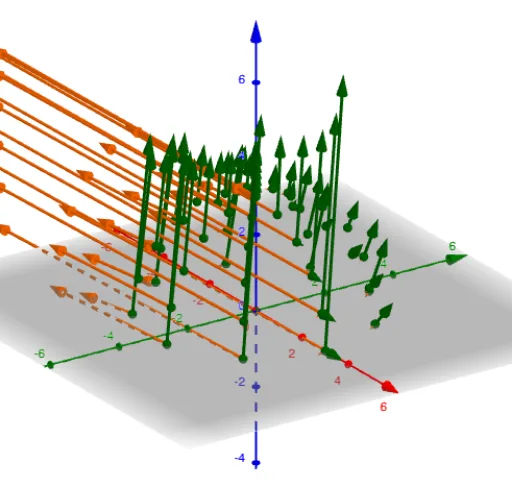
Loading the math board and drawing, please wait…
This example demonstrates the calculation and visualization of the curl of a vector field on a specific surface in 3D space. Key mathematical concepts include vector calculus, curl, 3D surfaces, vector fields, and parametric representation. The construction utilizes GeoGebra commands like Sequence, Derivative, and Textfield to dynamically generate the vector field, compute the curl, and display the results. It is suitable for university students in mathematics, physics, or engineering to understand vector field properties and the physical significance of curl.
GeoGebra Commands & Parameters
Sequence(Sequence[(((umax - umin) / xstep * i) + umin, ((vmax - vmin) / ystep * j) + vmin), i, 0, xstep], j, 0, ystep) → L_1Sequence(Sequence[(rx(L_1(j, i)), ry(L_1(j, i)), rz(L_1(j, i))), i, 1, xstep + 1], j, 1, ystep + 1) → L_2Sequence(Sequence[Vector[(rx(L_1(j, i)), ry(L_1(j, i)), rz(L_1(j, i))), (rx(L_1(j, i)), ry(L_1(j, i)), rz(L_1(j, i))) + (scaleF * (P(L_1(j, i)), Q(L_1(j, i)), R(L_1(j, i))))], i, 1, xstep + 1], j, 1, ystep + 1) → L_3Derivative(P, y) → PyDerivative(P, z) → PzDerivative(Q, x) → QxDerivative(Q, z) → QzDerivative(R, x) → RxDerivative(R, y) → RySequence(Sequence[Vector[(rx(L_1(j, i)), ry(L_1(j, i)), rz(L_1(j, i))), (rx(L_1(j, i)), ry(L_1(j, i)), rz(L_1(j, i))) + (scaleCurl * (Ry(L_1(j, i)) - Qz(L_1(j, i)), Pz(L_1(j, i)) - Rx(L_1(j, i)), Qx(L_1(j, i)) - Py(L_1(j, i))))], i, 1, xstep + 1], j, 1, ystep + 1) → L_4Textfield(umin) → InputBox1Textfield(umax) → InputBox2Textfield(vmin) → InputBox3Textfield(vmax) → InputBox4Textfield(rx) → InputBox5Textfield(ry) → InputBox6Textfield(rz) → InputBox7Textfield(P) → InputBox8Textfield(Q) → InputBox9Textfield(R) → InputBox10
AI Drawing Prompt Reference
Create a 3D parametric surface with a grid of points, and at each point display two vector fields: the original vector field with shorter arrows and its curl with longer arrows, both originating from the surface. The surface is defined by adjustable parameter ranges, and the vector field components are user-modifiable. The visualization should clearly show how the curl represents local rotation of the field on the surface, suitable for educational demonstration.
The prompt above was compiled from the original drawing commands and is for reference only.