
Cumulative Frequency Polygon Demonstration
Loading the math board and drawing, please wait…
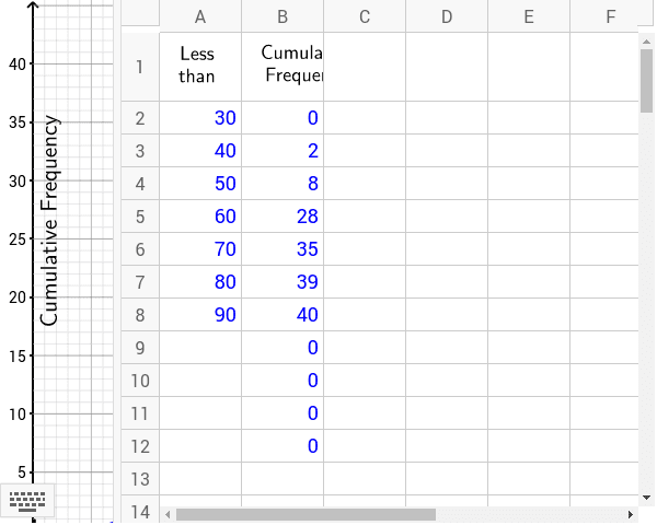
① This example demonstrates how to construct a cumulative frequency polygon, visualizing the cumulative distribution of a data set. ② Core concepts include cumulative frequency, frequency distribution, and polygon fitting in statistics. ③ Construction uses GeoGebra commands If, Sequence, PolyLine, Polygon, Point, Textfield, RotateText and objects such as yint2, xint2, A2, unitx, unity, list1, list2, poly1 to create vertices, axis scaling, and labels. ④ Suitable for high‑school statistics lessons, introductory university probability‑statistics courses, and teacher lesson‑plan references.
GeoGebra Commands & Parameters
If(A3 - A2 > 0, A3 - A2, 5) → kSequence((k * i, Element[list1, i]), i, 1, n) → list2PolyLine(list2) → aPolygon((unitx, 0.3), (unitx, -0.3), (2.5 * unitx, -0.3), (2.5 * unitx, 0.3)) → poly1, b, c, d, eSequence(Segment[(xmin + xint2 * i, ymax), (xmin + xint2 * i, ymin)], i, 1, (xmax - xmin) / xint2) → list3Sequence(Segment[(xmin + xint1 * i, ymax), (xmin + xint1 * i, ymin)], i, 1, (xmax - xmin) / xint1) → list5Sequence(Segment[(xmin, ymin + yint1 * i), (xmax, ymin + yint1 * i)], i, 1, (ymax - ymin) / yint1) → list6Sequence(Segment[(xmin, ymin + yint2 * i), (xmax, ymin + yint2 * i)], i, 1, (ymax - ymin) / yint2) → list4Point(Segment[(k, 0), (n * k, 0)]) → PPoint(Segment[(k, 0), (n * k, 0)]) → QPoint(Segment[(0, 0), (0, Element[list1, n])]) → P'Point(Segment[(0, 0), (0, Element[list1, n])]) → Q'PolyLine((unitx, 0), (1.5 * unitx, h), (2 * unitx, -h), (2.5 * unitx, 0)) → fSequence(Segment[(k * i, 0), (k * i, (-h) / 3)], i, 1, n) → list7PolyLine(P, Intersect[x = x(P), a], P_1) → iPolyLine(P', Intersect[y = y(P'), a], P'_1) → lPolyLine(Q, Intersect[x = x(Q), a], Q_1) → jPolyLine(Q', Intersect[y = y(Q'), a], Q'_1) → mTextfield(xint2) → inputBox2Textfield(yint2) → inputBox3Textfield(text15) → inputBox5Textfield(text16) → inputBox4RotateText("Cumulative Frequency", 90*°) → text18