
Cube Shadows Demonstration
Loading the math board and drawing, please wait…
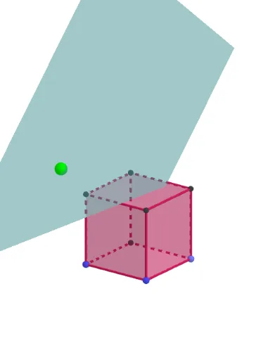
This example demonstrates the changing shadows of a cube under varying angles of light, involving concepts in solid geometry, projection transformations, and trigonometry (sine, cosine). Key GeoGebra commands/objects used include Point, Cube, Sphere, Line, OrthogonalPlane, OrthogonalLine, Intersect, and Polygon. Suitable for high school students studying solid geometry, spatial visualization, and geometric constructions.
GeoGebra Commands & Parameters
Point(Circle[(1, -1, -1), Distance[(-1, -1, -1), (1, -1, -1)], Segment[(-1, -1, -1), (1, -1, -1)]]) → ACube((-1, -1, -1), (1, -1, -1), A) → a, B, faceABFE, faceCDEF, edge2, edge1, edge4, edgeAB, edge3, edgeBF, edgeCF, edgeCD, C, edge5, edgeDE, edgeAE, edgeEF, D, E, F, face1, face3, face2, face4Sphere((0, 0, 0), 3) → bPointIn(b) → ILine(I, (0, 0)) → fOrthogonalPlane(I, f) → cOrthogonalLine(C, c) → gOrthogonalLine(F, c) → hOrthogonalLine(E, c) → iOrthogonalLine(B, c) → jOrthogonalLine(G, c) → kOrthogonalLine(H, c) → lOrthogonalLine(A, c) → mIntersect(i, c) → JIntersect(h, c) → KIntersect(m, c) → LIntersect(g, c) → MIntersect(l, c) → NIntersect(j, c) → OIntersect(k, c) → POrthogonalLine(D, c) → nIntersect(n, c) → QPolygon(M, K, O, P) → q1, m_1, k_1, o, pPolygon(Q, J, L, N) → q2, q, j_1, l_1, n_1Polygon(Q, M, K, J) → q3, q_1, m_2, k_2, j_2Polygon(L, O, K, J) → q4, l_2, o_1, k_3, j_3Polygon(Q, M, P, N) → q5, q_2, m_3, p_1, n_2Polygon(P, O, L, N) → q6, p_2, o_2, l_3, n_3
AI Drawing Prompt Reference
Draw a cube and observe how its shadow changes at different angles. Start by creating a cube, then create a light source point and a plane passing through this point. From each vertex of the cube, draw a perpendicular line to this plane and find the intersection points. Finally, connect these intersection points to form the shadow.
The prompt above was compiled from the original drawing commands and is for reference only.