
Critical Points of Volume Surface for the Eight-Point Model
Loading the math board and drawing, please wait…
In collections
₉Extreme Verteilung der 8 Punkten auf der Kugel
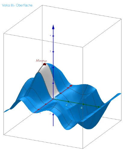
This example demonstrates the critical points of the volume surface in the eight-point model as parameters α and θ vary. It involves core mathematical concepts such as volume calculation, derivatives, extrema, 3D geometry, and parametric equations. GeoGebra commands like Function, Derivative, Plane, Polygon, Textfield, and Point are used to dynamically visualize volume changes and critical points. Suitable for high school students and math enthusiasts studying 3D function optimization and geometric modeling.
GeoGebra Commands & Parameters
Function(Vol(u, v), u, -1°, 60°, v, -1°, 90°) → mDerivative(Vol(x, y), x) → Vol_xDerivative(Vol(x, y), y) → Vol_yPlane(z = z0) → Plane0Polygon({(-1°, -1°), (60°, -1°), (60°, 90°), (-1°, 90°), (-1°, -1°)}) → Poly_{αθ}Plane(z = 1.539600717839) → Pl_{Lö1}Plane(z = 1.752175217161758) → Pl_{Lö2}Textfield(Δθ) → InputBox1Point(xAxis) → Ca4
AI Drawing Prompt Reference
Draw the volume surface of the eight-point model and find its critical points. First, plot the volume function V(u, v) for u from -1° to 60° and v from -1° to 90°. Then, calculate the partial derivatives of the volume function with respect to u and v to get Vol_x and Vol_y. Next, draw planes at z=1.539600717839 and z=1.752175217161758 as the critical points of the volume surface. Finally, draw a rectangular region representing the range of parameters α and θ, and mark a point Ca4 on the x-axis.
The prompt above was compiled from the original drawing commands and is for reference only.