
Critical Points as Geometric Medians and Hessian Matrix
Loading the math board and drawing, please wait…
In collections
₅Point Location estimators: Geometric Medians on a sphere
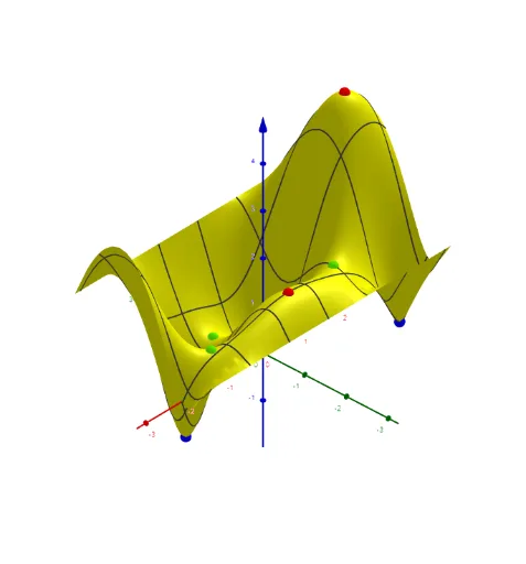
This example explores the nature of critical points using the concept of geometric medians and the Hessian matrix. It first constructs a series of geometric objects, such as points and line segments, to demonstrate how to find the critical points of a function. Then, it uses the Hessian matrix to determine the nature of these critical points, such as whether they are maxima, minima, or saddle points. The example utilizes commands like Polygon, PointIn, Sequence, Zip, and TableText in GeoGebra, making it suitable for high school mathematics teachers and students studying calculus and optimization problems.
GeoGebra Commands & Parameters
Polygon({((-π), ((-π)) / 2), ((-π), π / 2), (π, π / 2), (π, ((-π)) / 2)}) → qPointIn(q) → P9PointIn(q) → A_2Sequence(If[D(i) > 0, If[f_{xx}(i) > 0, "local minimum", "local maximum"], If[(D(i) * f_{xx}(i)) ≟ 0, "?", "saddle point"]], i, 1, Length[l1]) → l4Zip((x(a), y(a)), a, l1) → l5TableText(Append["i", 1…Length[l1]], Append["critical points", l5], Append["f_{x}", lfx], Append["f_{y}", lfy], Append["f_{xx}", f_{xx}], Append["Det", D], Append["", l4], "v") → text1Function((q_f * f(u, v)) + b_0, u, (-π), π, v, ((-π)) / 2, π / 2) → f0Length(lsad) → läsadLength(lmax) → lämaxLength(lmin) → läminZip(Segment[A, p], p, lP) → segSum(seg) → sum_segFlatten(Sequence[Sequence[((-π) + ((2 * π / na) * i), ((-π)) / 2 + (π / na * j)), j, 1, na - 1], i, 1, na - 1]) → ltest_2Zip((R; x(a); y(a)), a, ltest_2) → ltest_3TableText(Append["i", Sequence[Length[lmax]]], Append["P_{Max }\;(φ,θ)", lmax], Append["(f'x,f'y)", lZf'xymax], "v") → textmaxTableText(Append["i", Sequence[Length[(lmin * x)]]], Append["P_{Max }\;(φ,θ)", lmin], Append["(f'x,f'y)", lZf'xymin], "v") → textminTableText(Append["i", Sequence[Length[(lsad * x)]]], Append["P_{Max }\;(φ,θ)", lsad], Append["(f'x,f'y)", lZf'xysad], "v") → textsadTextfield(R) → InputBox1Textfield(n) → InputBox2Textfield(lP) → InputBox3
AI Drawing Prompt Reference
Draw a rectangular region with x from -π to π and y from -π/2 to π/2. Place two random points inside. Generate a grid of test points. Display a function surface over the region. Mark critical points and list them in a table with coordinates, first and second partial derivatives, and determinant, classifying each as local maximum, minimum, or saddle. Connect each critical point to a reference point with line segments and show their total length. Include three input fields for adjusting radius, number of points, and reference point set.
The prompt above was compiled from the original drawing commands and is for reference only.