
Creating a Histogram from a Table in GeoGebra
Loading the math board and drawing, please wait…
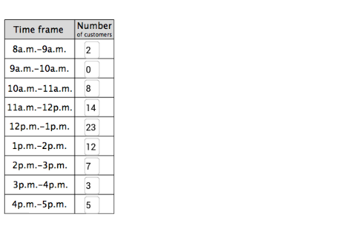
This example demonstrates how to create a histogram from a table in GeoGebra, visually displaying the frequency distribution of a dataset and its step-function outline. The core mathematical concepts include histograms, statistical distributions, step functions, data binning, frequency characteristics, and boxplot-related statistical features. The construction uses GeoGebra commands such as Textfield, Polygon, Segment, Sequence, Vector, Sort, Element, and If, along with objects including t0, t1, t2, directions1, d1, inputD1, directions3, directions2, tableHeader, xMin, xMax, yMin, yMax, header1, and table cells table11 through table18 to control table input, interval boundaries, rectangular bars, and step segments. It is suitable for high school probability and statistics instruction and for introductory college statistics courses that require interactive data visualization and exploratory learning.
GeoGebra Commands & Parameters
Textfield(d1) → inputD1Polygon((0, 11), (If[showSteps > t0, t1, t2], 11), (If[showSteps > t0, t1, t2], 12), (0, 12)) → tableHeader, b, c, d, eSegment((0, 10), (If[showSteps > t0, t1, t2], 10)) → fSegment((0, 9), (If[showSteps > t0, t1, t2], 9)) → gSegment((0, 8), (If[showSteps > t0, t1, t2], 8)) → hSegment((0, 7), (If[showSteps > t0, t1, t2], 7)) → iSegment((0, 6), (If[showSteps > t0, t1, t2], 6)) → jSegment((0, 5), (If[showSteps > t0, t1, t2], 5)) → kSegment((0, 4), (If[showSteps > t0, t1, t2], 4)) → lSegment((0, 3), (If[showSteps > t0, t1, t2], 3)) → mSegment((t1, 0), (t1, 12)) → sTextfield(d2) → inputD2Textfield(d3) → inputD3Textfield(d4) → inputD4Textfield(d5) → inputD5Textfield(d6) → inputD6Textfield(d7) → inputD7Textfield(d8) → inputD8Segment((0, 2), (If[showSteps > t0, t1, t2], 2)) → aTextfield(d9) → inputD9Segment((3.2, 2), (3.2, 12)) → qSegment((0, 2), (0, 11)) → nSegment((If[showSteps > t0, t1, t2], 2), (If[showSteps > t0, t1, t2], 11)) → pSequence(Segment[(i, -0.3), (i, 0)], i, 7, 18) → xAxisHashMarksVector((10, 0), (18.8, 0)) → xAxisRVector((10, 0), (6.2, 0)) → xAxisLVector((7, 2), (7, -0.8)) → yAxisBSort({d1, d2, d3, d4, d5, d6, d7, d8, d9}) → orderedElement(ordered, 9) → grIf(gr < 12, 1, If[gr < 24, 2, If[gr < 30, 3, If[gr < 60, 4, 5]]]) → ySetSequence(Segment[(i, 0), (i, 12)], i, 8, 1000) → gridVSequence(Segment[(7, i), (1000, i)], i, 1, 12) → gridHVector((7, 2), (7, 12.8)) → yAxisTSequence(Segment[(6.7, i), (7, i)], i, 1, 12) → yAxisHashMarksIf(ySet ≟ 1, 1, If[ySet ≟ 2, 2, If[ySet ≟ 3, 2.5, If[ySet ≟ 4, 5, 10]]]) → scaleFactorPolygon((8, 0), (9, 0), (9, d1 / scaleFactor), (8, d1 / scaleFactor)) → hist89, t, a_1, b_1, c_1Polygon((9, 0), (10, 0), (10, d2 / scaleFactor), (9, d2 / scaleFactor)) → hist910, d_1, e_1, f_1, g_1Polygon((10, 0), (11, 0), (11, d3 / scaleFactor), (10, d3 / scaleFactor)) → hist1011, h_1, i_1, j_1, k_1Polygon((11, 0), (12, 0), (12, d4 / scaleFactor), (11, d4 / scaleFactor)) → hist1112, l_1, m_1, n_1, p_1Polygon((12, 0), (13, 0), (13, d5 / scaleFactor), (12, d5 / scaleFactor)) → hist121, q_1, r_1, s_1, t_1Polygon((13, 0), (14, 0), (14, d6 / scaleFactor), (13, d6 / scaleFactor)) → hist12, a_2, b_2, c_2, d_2Polygon((14, 0), (15, 0), (15, d7 / scaleFactor), (14, d7 / scaleFactor)) → hist23, e_2, f_2, g_2, h_2Polygon((15, 0), (16, 0), (16, d8 / scaleFactor), (15, d8 / scaleFactor)) → hist34, i_2, j_2, k_2, l_2Polygon((16, 0), (17, 0), (17, d9 / scaleFactor), (16, d9 / scaleFactor)) → hist45, m_2, n_2, p_2, q_2
AI Drawing Prompt Reference
Draw a histogram built from a table of nine values: nine equal-width bars whose heights are the entered frequencies scaled by the maximum value, a step-function outline connecting the bar tops, horizontal and vertical axes with tick marks and a full grid, and on the left a column of nine editable input fields for the raw frequencies together with a header row and guiding segments. The layout proceeds from the data entry area on the left to the coordinate system and grid, then to the histogram bars and step outline on the right.
The prompt above was compiled from the original drawing commands and is for reference only.