
Coupled Differential Equations Demo
Loading the math board and drawing, please wait…
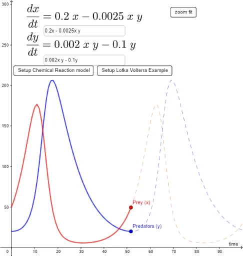
This example demonstrates the numerical solutions and trajectories of coupled differential equations. Key math concepts include differential equations, numerical methods, trajectory analysis, and linear systems. GeoGebra commands used are SolveODE for solving ODEs, Sequence and Ray for trajectory plotting, Point and Textfield for displaying solution points, Max and Min for range determination, and Segment and Intersect for auxiliary constructions. Suitable for high school students and math enthusiasts learning about differential equations and visualization.
GeoGebra Commands & Parameters
SolveODE(g, f, x(A), y(A), maxT, stepsolve) → ppsolSequence(x(Point[ppsol, tt]), tt, 0, 1, stepplot) → xlistSequence(y(Point[ppsol, tt]), tt, 0, 1, stepplot) → ylistRay((0, 0), (1, 0)) → hRay((0, 0), (0, 1)) → iPoint(ppsol, t / maxT) → BTextfield(f) → InputBox1Textfield(g) → InputBox2Sequence(Sequence[Vector[(ii, jj), (ii, jj) + (((y(D) - y(C)) / n * 0.5) * UnitVector[(f(ii, jj), g(ii, jj))])], ii, x(C), x(D), W / n], jj, y(C), y(D), H / n) → l1Max(xlist) → mxvalMax(ylist) → myvalMin(xlist) → mixvalMin(ylist) → miyvalSegment((x(B), 0), B) → jSegment((0, y(B)), B) → kIntersect(yAxis, k) → EIntersect(xAxis, j) → F
AI Drawing Prompt Reference
Draw a graph demonstrating the numerical solutions and trajectories of coupled differential equations, featuring rays extending from the origin along the x-axis and y-axis, and trajectories plotted based on the differential equation's numerical solution, with points connected by line segments to the coordinate axes, and labeled maximum and minimum points on the axes.
The prompt above was compiled from the original drawing commands and is for reference only.