
Optimal Cannon Launch Angle for Maximum Range at Various Ground Heights
Loading the math board and drawing, please wait…
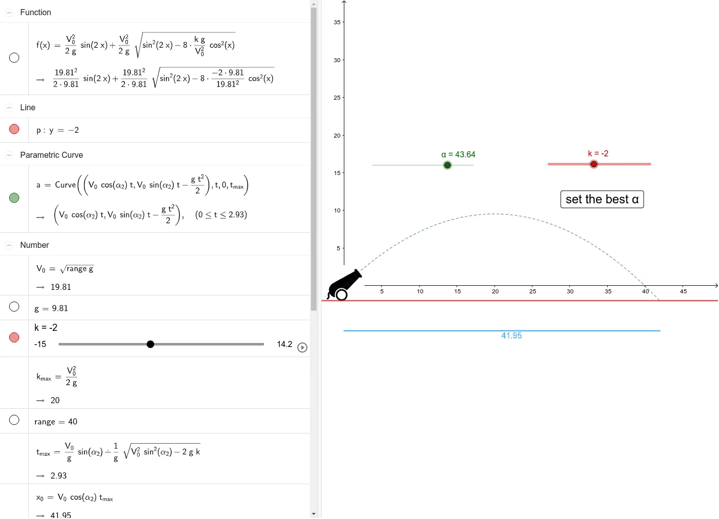
This GeoGebra example demonstrates how a cannonball's trajectory and horizontal range change with launch angle across different ground heights, dynamically identifying the optimal firing angle that maximizes distance. Core mathematical concepts include projectile motion kinematics, trigonometric and quadratic modeling, analytic geometry, and calculus-based optimization using derivatives to locate extrema. Construction highlights from the source summary include the Intersect command for intersection points, CurveCartesian for Cartesian curves, Point and Segment for geometric elements, Dilate and Rotate for scaling and rotation transformations, and Extremum for finding maximum range; relevant objects are initial velocity V₀, launch angle α, gravitational acceleration g, ground height h, range, maximum time tmax, and extremum points A, B, C, D. The resource is suitable for high school physics and mathematics interdisciplinary teaching, university calculus or analytic geometry courses, optimization modeling projects, and interactive parametric animation demonstrations.
GeoGebra Commands & Parameters
Intersect(xAxis, yAxis) → ACurveCartesian((((V_{0} * cos(α_{2})) * t), ((V_{0} * sin(α_{2})) * t) - ((g * t^(2))) / 2), t, 0, t_{max}) → aPoint(yAxis) → BPoint(Circle[B, x_{0}]) → CSegment(B, C) → hDilate(obraz1, 0.1, A) → obraz1'Rotate(obraz1', 10° + α° - 45°, A) → obraz1''Extremum(f, (-(π / 2)), π / 2) → D
AI Drawing Prompt Reference
Create a parametric projectile-motion visualization showing how the horizontal range changes with launch angle across different ground heights. Draw coordinate axes, then plot the cannonball trajectory using x=V0·cos(α)·t and y=V0·sin(α)·t−g·t^2/2 for t from 0 to the maximum time tmax. Include a reference point on the vertical axis and connect it with a segment representing the ground height h. Apply a scaling transformation to the trajectory and then rotate the scaled trajectory about the reference point to depict the angle-dependent variation. Finally, mark an extremum point D for the function f on the interval (−π/2, π/2), indicating the launch angle that yields the maximum range.
The prompt above was compiled from the original drawing commands and is for reference only.