
Coupled Differential Equations Demo by Ben Sparks
Loading the math board and drawing, please wait…
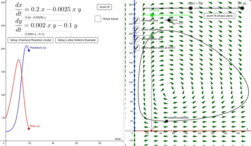
This example demonstrates the numerical solutions and trajectories of coupled differential equations. Key math concepts include differential equations, numerical methods, parametric equations, and function graphing. Construction highlights involve SolveODE for solving ODEs, Sequence and Ray for trajectory creation, Point and Textfield for displaying solutions, Max and Min for range determination, and Segment and Intersect for auxiliary lines. Suitable for high school students and math enthusiasts learning about differential equation visualization and numerical solutions.
GeoGebra Commands & Parameters
SolveODE(g, f, x(A), y(A), maxT, stepsolve) → ppsolSequence(x(Point[ppsol, tt]), tt, 0, 1, stepplot) → xlistSequence(y(Point[ppsol, tt]), tt, 0, 1, stepplot) → ylistRay((0, 0), (1, 0)) → hRay((0, 0), (0, 1)) → iPoint(ppsol, t / maxT) → BTextfield(f) → InputBox1Textfield(g) → InputBox2Sequence(Sequence[Vector[(ii, jj), (ii, jj) + (((y(D) - y(C)) / n * 0.5) * UnitVector[(f(ii, jj), g(ii, jj))])], ii, x(C), x(D), W / n], jj, y(C), y(D), H / n) → l1Max(xlist) → mxvalMax(ylist) → myvalMin(xlist) → mixvalMin(ylist) → miyvalSegment((x(B), 0), B) → jSegment((0, y(B)), B) → kIntersect(yAxis, k) → EIntersect(xAxis, j) → F