Comparing Numerical Integration: Upper/Lower Riemann Sums and Trapezoids

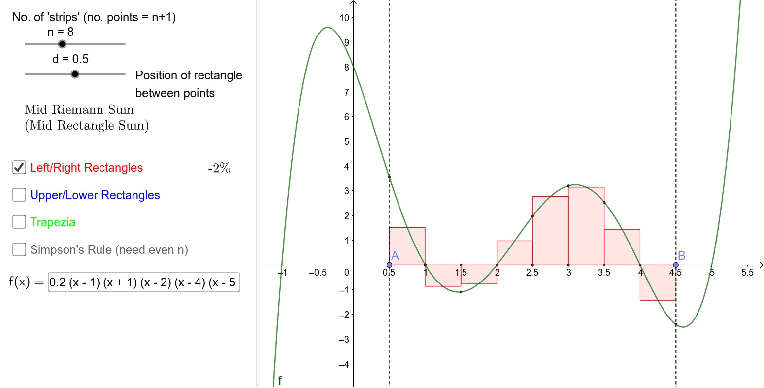
This GeoGebra example visualizes numerical integration by comparing geometric area approximations of a function over [A,B]. It demonstrates how the upper and lower Riemann sums, as well as the trapezoidal sum, approximate the definite integral and how the approximation improves as the number of subintervals increases. The key math concepts include the definite integral, UpperSum and LowerSum (upper/lower Riemann sums), TrapezoidalSum, partitioning the interval, and the role of discretization in numerical accuracy. Construction highlights: Points and RectangleSum are used to build the rectangle-based area visualization; If and Sequence help generate piecewise parameters and summation terms; UpperSum, LowerSum, and TrapezoidalSum produce Upsum, Lowsum, and Trapsum; Sum and Integral enable a direct comparison between the numerical approximations and the exact definite integral. Textfield labels and annotations (e.g., for interval endpoints and mid/left/right information) support clear interpretation. Suitable for high school and early calculus courses, as well as learners studying the geometric meaning of integrals and basic numerical integration methods.