
Correlation Analysis of Height and Free Throw Percentage
Loading the math board and drawing, please wait…
In collections
CCSS IP Math I Unit 4 Lesson 3
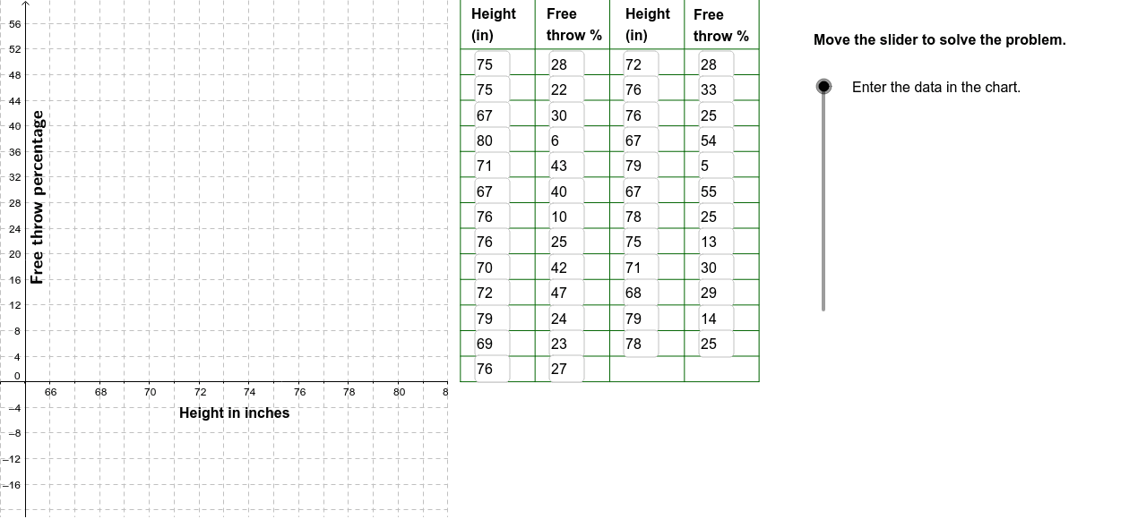
This GeoGebra example demonstrates the correlation between basketball players' height and free throw shooting percentage using scatter plots and function graphs. Key math concepts include Pearson correlation coefficient (PMCC), linear fitting (FitLineY), and statistical visualization. Construction involves commands like FitLineY for line fitting, PMCC for correlation calculation, Textfield for labels, and Polygon, Sequence, Segment, RotateText for geometric elements and data sequences. Suitable for high school or college statistics courses to teach correlation and regression analysis.
GeoGebra Commands & Parameters
FitLineY(PointList1) → LineFitPMCC(PointList1) → CorCoeffTextfield(A2) → InA2Textfield(A3) → InA3Textfield(A4) → InA4Textfield(A5) → InA5Textfield(A6) → InA6Textfield(A7) → InA7Textfield(A8) → InA8Textfield(A9) → InA9Textfield(A10) → InA10Textfield(A11) → InA11Textfield(A12) → InA12Textfield(A13) → InA13Textfield(A14) → InA14Textfield(A15) → InA15Textfield(A16) → InA16Textfield(A17) → InA17Textfield(A18) → InA18Textfield(A19) → InA19Textfield(A20) → InA20Textfield(A21) → InA21Textfield(B2) → InB2Textfield(B3) → InB3Textfield(B4) → InB4Textfield(B5) → InB5Textfield(B6) → InB6Textfield(B7) → InB7Textfield(B8) → InB8Textfield(B9) → InB9Textfield(B10) → InB10Textfield(B11) → InB11Textfield(B12) → InB12Textfield(B13) → InB13Textfield(B14) → InB14Textfield(B15) → InB15Textfield(B16) → InB16Textfield(B17) → InB17Textfield(B18) → InB18Textfield(B19) → InB19Textfield(B20) → InB20Textfield(B21) → InB21Polygon((82, y(Corner[1])), Corner[2], Corner[3], (82, y(Corner[4]))) → poly1, a, b, c, dTextfield(A22) → InA22Textfield(A23) → InA23Textfield(A24) → InA24Textfield(A25) → InA25Textfield(A26) → InA26Textfield(B22) → InB22Textfield(B23) → InB23Textfield(B24) → InB24Textfield(B25) → InB25Textfield(B26) → InB26Sequence(Segment[(82.5, 0 + (4 * i)), (94.5, 0 + (4 * i))], i, 0, 13) → Linesh1Sequence(Segment[(82.5 + (3 * i), 0), (82.5 + (3 * i), 60)], i, 0, 4) → Linesv1Segment((82.5, 59.9), (94.5, 59.9)) → top1RotateText("Free throw percentage", 90*°) → SideLegend
AI Drawing Prompt Reference
Create a scatter plot showing the relationship between basketball players' heights and their free throw shooting percentages. Add a linear regression line that best fits the data points, and compute the Pearson correlation coefficient to quantify the strength and direction of the correlation. Display the coefficient value on the graph. Include text labels for each data point indicating its height and corresponding free throw percentage. Finally, draw a polygon region on the right side of the plot to highlight the area of interest, such as a confidence band or annotation zone.
The prompt above was compiled from the original drawing commands and is for reference only.