
Contour Plot Guide
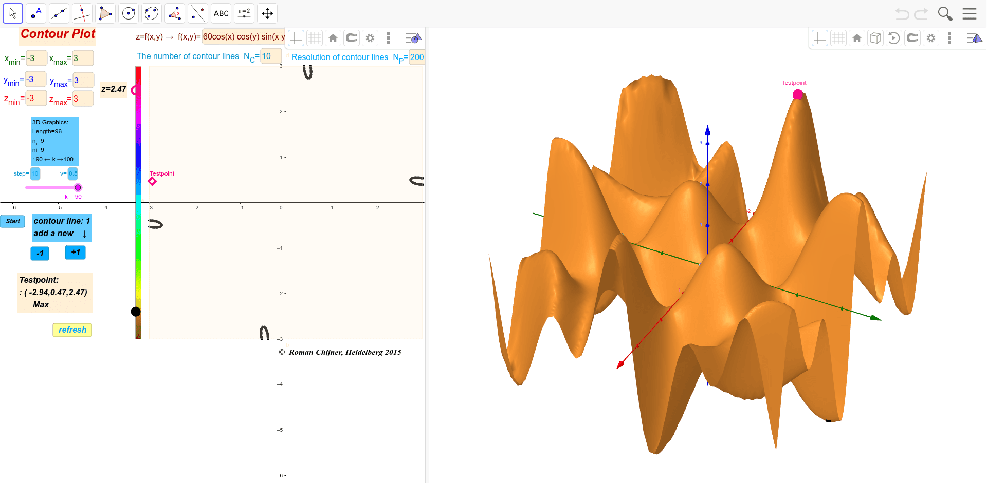
Loading the math board and drawing, please wait…
This example demonstrates how to create contour plots for arbitrary functions z=f(x,y). Key mathematical concepts include function graphs, contour lines, and coordinate systems. Construction involves GeoGebra commands like Polygon, Segment, RemoveUndefined, etc. Suitable for high school students or college freshmen learning function visualization and spatial geometry.
GeoGebra Commands & Parameters
Polygon((x_{min}, y_{min}), (x_{max}, y_{min}), (x_{max}, y_{max}), (x_{min}, y_{max})) → poly1, b, c, d, eSegment(B02, B01) → aRemoveUndefined(Join[Zip[Mirror[{Roots[f0(a, x), y_{min}, y_{max}]}, y = x] + (a, 0), a, Sequence[x_{min} + ((x_{max} - x_{min}) / N_P * i), i, 0, N_P]]]) → P1xxyRemoveUndefined(Join[Zip[Reverse[{Roots[f0(x, a), x_{min}, x_{max}]}] + (0, a), a, Sequence[y_{min} + ((y_{max} - y_{min}) / N_P * i), i, 0, N_P]]]) → P2yyxTextfield(v_1) → inputBox2Textfield(f) → inputBox3Textfield(N_C) → inputBox1Textfield(x_{min}) → inputBox4Textfield(x_{max}) → inputBox5Textfield(y_{max}) → inputBox6Textfield(z_{max}) → inputBox7Textfield(y_{min}) → inputBox8Textfield(z_{min}) → inputBox9PointIn(poly1) → PTestPoint(a, 1 - zzii_B) → ATextfield(N_P) → inputBox10Sum(Sequence[If[f0(x(PTest), y(PTest)) - f0(x(Element[lr01, i]), y(Element[lr01, i])) > 0, 1, 0], i, 1, 11]) → ext1Zip((x(a), y(a), z0), a, Join[{P1xxy, P2yyx}]) → list1Length(list1) → LäTextfield(v) → inputBox11Textfield(step) → inputBox12Sequence(Element[list1, i], i, k, k + step) → M01Function(f(a, b), a, x_{min} - 0.2, x_{max} + 0.2, b, y_{min} - 0.2, y_{max} + 0.2) → g