
Contour of Saddle Surface in Axonometry 2
Loading the math board and drawing, please wait…
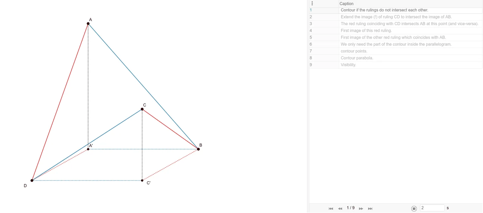
This example demonstrates the contour lines of a saddle surface in axonometric projection. Key mathematical concepts include surfaces, axonometric projection, and geometric construction. It utilizes commands like Segment, Line, Intersect, OrthogonalLine, Point, Locus, and Polygon in GeoGebra to create the visualization. Suitable for high school and above students studying 3D geometry and projection transformations.
GeoGebra Commands & Parameters
Segment(D, A') → fSegment(A', B) → gLine(B, f) → hLine(D, g) → iIntersect(h, i) → C'Segment(D, C') → jSegment(C', B) → kOrthogonalLine(A', g) → lOrthogonalLine(C', j) → mPoint(l) → APoint(m) → CSegment(A, A') → nSegment(C, C') → pSegment(D, A) → qSegment(A, B) → rSegment(B, C) → sSegment(C, D) → tLine(D, C) → s_2Intersect(s_2, r) → ESegment(C, E) → aLine(E, n) → bIntersect(i, b) → FIntersect(g, b) → GSegment(E, F) → f_1Segment(F, C') → cLine(F, k) → dLine(B, j) → eIntersect(d, e) → HSegment(F, H) → g_1Segment(H, B) → h_1Line(G, k) → i_1Intersect(j, i_1) → ISegment(G, I) → j_1Segment(H, I) → k_1Intersect(k, k_1) → JLine(I, n) → l_1Line(J, l_1) → m_1Intersect(t, l_1) → KIntersect(s, m_1) → LSegment(K, I) → q_1Segment(L, J) → t_1Segment(J, I) → a_1Point(a_1) → MLine(M, j_1) → c_1Intersect(j, c_1) → NIntersect(c_1, g) → OLine(N, n) → d_1Line(O, d_1) → e_1Segment(K, I) → n_1Intersect(d_1, t) → PIntersect(e_1, r) → QSegment(P, Q) → f_2Line(M, n) → g_2Intersect(g_2, f_2) → RLocus(R, M) → ponthalmaz1Segment(L, J) → p_1Segment(D, C) → r_1Segment(C, B) → s_1Segment(A, D) → b_1Intersect(r_1, b_1) → TIntersect(r_1, s_1) → UPoint(r_1) → VIntersect(h_1, s_1) → SSegment(A, S) → h_2Intersect(b_1, h_2) → WPolygon(D, U, S, W) → q1, d_2, u, s_3, wPoint(ponthalmaz1) → ZPoint(ponthalmaz1) → A_1Point(ponthalmaz1) → B_1Point(ponthalmaz1) → C_1Point(ponthalmaz1) → D_1Point(ponthalmaz1) → E_1Point(ponthalmaz1) → F_1Point(ponthalmaz1) → G_1Point(ponthalmaz1) → H_1Polygon(U, S, G_1, H_1, K, L, Z, A_1, B_1, C_1, D_1, E_1, F_1) → poligon1, u_1, p_2, q_2, r_2, k_3, s_4, l_2, z_1, i_2, j_2, k_2, m_2, n_2
AI Drawing Prompt Reference
Draw an axonometric projection of a saddle surface showing its contour lines. Start with a quadrilateral base and its projection. From two base vertices, erect perpendiculars to define two elevated points, forming the surface edges. On the projection plane, use intersections and auxiliary lines to construct the main contour lines, then generate inner contours by connecting intersection points with parallels, completing the saddle-shaped outline.
The prompt above was compiled from the original drawing commands and is for reference only.