
Connectivity Matrix by chris cambré (3)
Loading the math board and drawing, please wait…
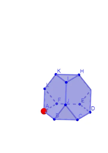
This example illustrates the concept of a connectivity matrix, involving core mathematical concepts of matrices and graph theory. Using GeoGebra commands such as Circle, Intersect, Rotate, etc., a complex geometric figure is constructed. This example is suitable for high school students or math enthusiasts learning about matrices and graph theory.
GeoGebra Commands & Parameters
Circle(OO, 1, xOyPlane) → cIntersect(yAxis, c, 2) → ARotate(A, 60°) → BRotate(A, 120°) → CRotate(A, 180°) → DRotate(A, 240°) → ERotate(A, 300°) → FPolygon(A, B, C, D, E, F) → veelhoek1, a, b, c_1, d, e, fPolygon(B, A, 6, xOyPlane) → veelhoek2, g, J_1, h, i, j, k, l, G_1, H_1, I_1Polygon(D, C, 6, xOyPlane) → veelhoek3, m, N, n_1, p, q, r, s, K_1, L_1, MPolygon(F, E, 6, xOyPlane) → veelhoek4, t, R, f_1, g_1, h_1, i_1, j_1, O, P, QCircle(c_1, K_1) → d_1Circle(a, J_1) → e_1Intersect(e_1, d_1) → J, T, ,Line(D, C) → k_1OrthogonalLine(K_1, k_1, xOyPlane) → l_1Intersect(k_1, l_1) → KKAngle(K_1, KK, J) → αRotate(veelhoek3, (-α), c_1) → veelhoek3'Line(OO, OOO) → asRotate(veelhoek3', 120°, as) → veelhoek3''Rotate(veelhoek3', (-(120°)), as) → veelhoek3''_1Rotate(J, (-(120°)), as) → LRotate(J, 120°, as) → GMidpoint(L, J) → UOrthogonalLine(U, veelhoek3''_1) → mmRotate(J, (-(60°)), mm) → IRotate(I, 120°, as) → HRotate(I, (-(120°)), as) → KPolygon(D, E, G) → driehoek1, s'_1, d_2, e_2Rotate(driehoek1, 120°, as) → driehoek1'Rotate(driehoek1, (-(120°)), as) → driehoek1'_1Point(vlakken3) → PPPTableText({{"A", "B", "C", "D", "E", "F", "G", "H", "I", "J", "K", "L"}}) → tekst1TableText({{"A"}, {"B"}, {"C"}, {"D"}, {"E"}, {"F"}, {"G"}, {"H"}, {"I"}, {"J"}, {"K"}, {"L"}}) → tekst2