
Sarrus’ Rule for a 3×3 Determinant—Geometric Construction
Loading the math board and drawing, please wait…
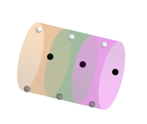
This example demonstrates how to compute a 3×3 determinant using Sarrus’ Rule in a visual, construction-based way. It builds a geometrical/table-like layout where the determinant is obtained from the products of three downward-diagonal terms minus the products of three upward-diagonal terms, making the sign pattern and term pairing easy to read. The key mathematics includes 3rd-order determinants, the arrangement of matrix coefficients into diagonal terms, and the positive/negative structure of the Sarrus expansion. In GeoGebra, the construction is driven by commands such as TableText to organize coefficient entries, Segment to draw the core structural lines, Translate and Rotate to replicate shifted/rotated components that correspond to diagonal term positions, and CurveCartesian to render coordinate-linked curves if needed for the visualization. Additional commands like Circle and Cylinder support auxiliary visual emphasis of the configuration, while Length can be used for geometric measurements related to the setup. The final determinant value is computed with the det operation, using explicitly constructed intermediate objects (e.g., the various d*, r*, c* sets) to correspond to the determinant’s diagonal product terms. Suitable for high school and early undergraduate linear algebra, especially for classroom demonstrations and conceptual understanding of determinant computation.
GeoGebra Commands & Parameters
TableText(M, "vc", 100, 100) → tabSegment((-3, 6) + ((-s), s), (3, 0) + (s, (-s))) → d1bCircle(Point[d1b, t], r) → c1Segment((-3, 4) + ((-r), r), (3, -2) + (r, (-r))) → d2bCircle(Point[d2b, t - 2], r) → c2Translate(c2, (0, 6)) → c2'Segment((-3, 6), Point[d1b, t]) → r1bSegment((-3, 2) + ((-r), r), (3, -4) + (r, (-r))) → d3bCircle(Point[d3b, t - 4], r) → c3Translate(c3, (0, 6)) → c3'Segment((-3, 4), If[y(Point[d2b, t - 2]) > 0, Point[d2b, t - 2], (1, 0)]) → r2bSegment(If[y(Point[d2b, t - 2]) > 0, Point[d2b, t - 2], (1, 6)], (0, 6) + Point[d2b, t - 2]) → r2b'Segment((-3, 2), If[y(Point[d3b, t - 4]) > 0, Point[d3b, t - 4], (-1, 0)]) → r3bSegment(If[y(Point[d3b, t - 4]) > 0, Point[d3b, t - 4], (-1, 6)], (0, 6) + Point[d3b, t - 4]) → r3b'Segment((3, 6) + (s, s), (-3, 0) + ((-s), (-s))) → d4bSegment((3, 4) + (r, r), (-3, -2) + ((-r), (-r))) → d5bSegment((3, 2) + (r, r), (-3, -4) + ((-r), (-r))) → d6bCircle(Point[d4b, t - 6], r) → c4Segment((3, 6), Point[d4b, t - 6]) → r4bCircle(Point[d5b, t - 8], r) → c5Segment((3, 4), If[y(Point[d5b, t - 8]) > 0, Point[d5b, t - 8], (-1, 0)]) → r5bSegment(If[y(Point[d5b, t - 8]) > 0, Point[d5b, t - 8], (-1, 6)], (0, 6) + Point[d5b, t - 8]) → r5b'Translate(c5, (0, 6)) → c5'Circle(Point[d6b, t - 10], r) → c6Segment((3, 2), If[y(Point[d6b, t - 10]) > 0, Point[d6b, t - 10], (1, 0)]) → r6bSegment(If[y(Point[d6b, t - 10]) > 0, Point[d6b, t - 10], (1, 6)], (0, 6) + Point[d6b, t - 10]) → r6b'Translate(c6, (0, 6)) → c6'Segment((-2.5, 5.5), (2.5, 0.5)) → d1aSegment((2.5, 5.5), (-2.5, 0.5)) → d4aTranslate(d1a, (0, -2)) → d2aTranslate(d1a, (0, -4)) → d3aTranslate(d4a, (0, -2)) → d5aTranslate(d4a, (0, -4)) → d6aSegment(Point[d1a, 0], Point[d1a, t]) → r1aSegment(Point[d2a, 0], Point[d2a, t - 2]) → r2aSegment(Point[d3a, 0], Point[d3a, t - 4]) → r3aSegment(Point[d4a, 0], Point[d4a, t - 6]) → r4aSegment(Point[d5a, 0], Point[d5a, t - 8]) → r5aSegment(Point[d6a, 0], Point[d6a, t - 10]) → r6aTableText(M', "vc", 100, 100) → tab'Translate((-3.06, 6.06), ((0, -6) * Min[t + 1, 1])) → Pu1Length(t4) → l4Length(t5) → l5Length(t6) → l6CurveCartesian((3 * k / pi) - 2, (-2 * sin(k + (2 * pi / 3))), (2 * cos(k + (2 * pi / 3))), k, 0, ((4 * pi / 3) * Min[1, t - 2])) → h2CurveCartesian((3 * k / pi) - 2, (-2 * sin(k + (4 * pi / 3))), (2 * cos(k + (4 * pi / 3))), k, 0, ((4 * pi / 3) * Min[1, t - 4])) → h3CurveCartesian((-3 * k / pi) + 2, (-2 * sin(k)), (2 * cos(k)), k, 0, ((4 * pi / 3) * Min[1, t - 6])) → h4CurveCartesian((-3 * k / pi) + 2, (-2 * sin(k + (2 * pi / 3))), (2 * cos(k + (2 * pi / 3))), k, 0, ((4 * pi / 3) * Min[1, t - 8])) → h5CurveCartesian((-3 * k / pi) + 2, (-2 * sin(k + (4 * pi / 3))), (2 * cos(k + (4 * pi / 3))), k, 0, ((4 * pi / 3) * Min[1, t - 10])) → h6CurveCartesian((3 * k / pi) - 2, (-2 * sin(k)), (2 * cos(k)), k, 0, ((4 * pi / 3) * Min[1, t])) → h1Rotate((-2, 0, 2), 120°, xAxis) → P_{2,1}Rotate((0, 0, 2), 120°, xAxis) → P_{2,2}Rotate((2, 0, 2), 120°, xAxis) → P_{2,3}Rotate((-2, 0, 2), 240°, xAxis) → P_{3,1}Rotate((0, 0, 2), 240°, xAxis) → P_{32}Rotate((2, 0, 2), 240°, xAxis) → P_{3,3}Cylinder((-2.5, 0, 0), (-2.5 + 5 / 3, 0, 0), 2) → a1, c, d, bCylinder((-2.5 + 5 / 3, 0, 0), (-2.5 + 10 / 3, 0, 0), 2) → a2, e, f, gCylinder((-2.5 + 10 / 3, 0, 0), (2.5, 0, 0), 2) → a3, h, k, i
AI Drawing Prompt Reference
Draw a 3x3 determinant using Sarrus' rule. First, create a 6x3 table and input the matrix elements. Then, draw two diagonals connecting the top-left to bottom-right and top-right to bottom-left. Next, draw circles and arcs around these diagonals to represent the determinant calculation process. Finally, use these circles and arcs to show the steps of the determinant calculation and display the determinant value.
The prompt above was compiled from the original drawing commands and is for reference only.