
Sarrus' Rule: Geometric Visualization of 3×3 Determinant Calculation
Loading the math board and drawing, please wait…
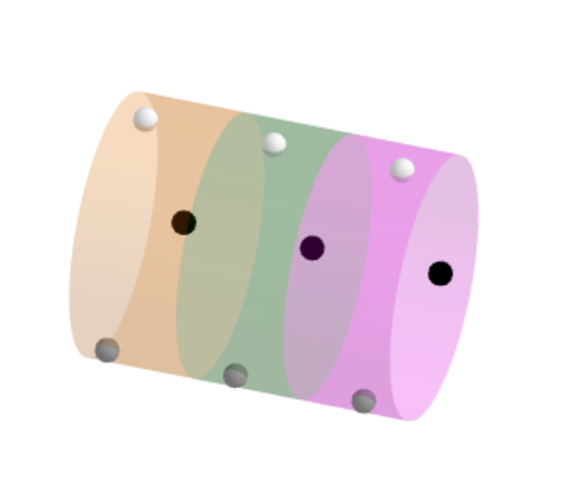
This example demonstrates Sarrus' rule for calculating a 3×3 determinant through geometric visualization. By mapping matrix elements to directed line segment lengths in a hexagonal diagram, it intuitively shows the calculation process of 'sum of products of main diagonals' minus 'sum of products of anti-diagonals'. Key mathematical concepts include determinant definition, matrix transformation, and geometric interpretation of vector cross product. Construction details: TableText creates the matrix table; Segment draws directed line segments; Circle builds the hexagonal auxiliary diagram; Translate and Rotate handle segment translation and rotation; Length measures segment lengths; Cylinder provides 3D visualization of results. Suitable for high school mathematics (introduction to determinants) and university linear algebra (matrices and determinants), helping students understand the geometric essence of determinant calculation.
GeoGebra Commands & Parameters
TableText(M, "vc", 100, 100) → tabSegment((-3, 6) + ((-s), s), (3, 0) + (s, (-s))) → d1bCircle(Point[d1b, t], r) → c1Segment((-3, 4) + ((-r), r), (3, -2) + (r, (-r))) → d2bCircle(Point[d2b, t - 2], r) → c2Translate(c2, (0, 6)) → c2'Segment((-3, 6), Point[d1b, t]) → r1bSegment((-3, 2) + ((-r), r), (3, -4) + (r, (-r))) → d3bCircle(Point[d3b, t - 4], r) → c3Translate(c3, (0, 6)) → c3'Segment((-3, 4), If[y(Point[d2b, t - 2]) > 0, Point[d2b, t - 2], (1, 0)]) → r2bSegment(If[y(Point[d2b, t - 2]) > 0, Point[d2b, t - 2], (1, 6)], (0, 6) + Point[d2b, t - 2]) → r2b'Segment((-3, 2), If[y(Point[d3b, t - 4]) > 0, Point[d3b, t - 4], (-1, 0)]) → r3bSegment(If[y(Point[d3b, t - 4]) > 0, Point[d3b, t - 4], (-1, 6)], (0, 6) + Point[d3b, t - 4]) → r3b'Segment((3, 6) + (s, s), (-3, 0) + ((-s), (-s))) → d4bSegment((3, 4) + (r, r), (-3, -2) + ((-r), (-r))) → d5bSegment((3, 2) + (r, r), (-3, -4) + ((-r), (-r))) → d6bCircle(Point[d4b, t - 6], r) → c4Segment((3, 6), Point[d4b, t - 6]) → r4bCircle(Point[d5b, t - 8], r) → c5Segment((3, 4), If[y(Point[d5b, t - 8]) > 0, Point[d5b, t - 8], (-1, 0)]) → r5bSegment(If[y(Point[d5b, t - 8]) > 0, Point[d5b, t - 8], (-1, 6)], (0, 6) + Point[d5b, t - 8]) → r5b'Translate(c5, (0, 6)) → c5'Circle(Point[d6b, t - 10], r) → c6Segment((3, 2), If[y(Point[d6b, t - 10]) > 0, Point[d6b, t - 10], (1, 0)]) → r6bSegment(If[y(Point[d6b, t - 10]) > 0, Point[d6b, t - 10], (1, 6)], (0, 6) + Point[d6b, t - 10]) → r6b'Translate(c6, (0, 6)) → c6'Segment((-2.5, 5.5), (2.5, 0.5)) → d1aSegment((2.5, 5.5), (-2.5, 0.5)) → d4aTranslate(d1a, (0, -2)) → d2aTranslate(d1a, (0, -4)) → d3aTranslate(d4a, (0, -2)) → d5aTranslate(d4a, (0, -4)) → d6aSegment(Point[d1a, 0], Point[d1a, t]) → r1aSegment(Point[d2a, 0], Point[d2a, t - 2]) → r2aSegment(Point[d3a, 0], Point[d3a, t - 4]) → r3aSegment(Point[d4a, 0], Point[d4a, t - 6]) → r4aSegment(Point[d5a, 0], Point[d5a, t - 8]) → r5aSegment(Point[d6a, 0], Point[d6a, t - 10]) → r6aTableText(M', "vc", 100, 100) → tab'Translate((-3.06, 6.06), ((0, -6) * Min[t + 1, 1])) → Pu1Length(t4) → l4Length(t5) → l5Length(t6) → l6CurveCartesian((3 * k / pi) - 2, (-2 * sin(k + (2 * pi / 3))), (2 * cos(k + (2 * pi / 3))), k, 0, ((4 * pi / 3) * Min[1, t - 2])) → h2CurveCartesian((3 * k / pi) - 2, (-2 * sin(k + (4 * pi / 3))), (2 * cos(k + (4 * pi / 3))), k, 0, ((4 * pi / 3) * Min[1, t - 4])) → h3CurveCartesian((-3 * k / pi) + 2, (-2 * sin(k)), (2 * cos(k)), k, 0, ((4 * pi / 3) * Min[1, t - 6])) → h4CurveCartesian((-3 * k / pi) + 2, (-2 * sin(k + (2 * pi / 3))), (2 * cos(k + (2 * pi / 3))), k, 0, ((4 * pi / 3) * Min[1, t - 8])) → h5CurveCartesian((-3 * k / pi) + 2, (-2 * sin(k + (4 * pi / 3))), (2 * cos(k + (4 * pi / 3))), k, 0, ((4 * pi / 3) * Min[1, t - 10])) → h6CurveCartesian((3 * k / pi) - 2, (-2 * sin(k)), (2 * cos(k)), k, 0, ((4 * pi / 3) * Min[1, t])) → h1Rotate((-2, 0, 2), 120°, xAxis) → P_{2,1}Rotate((0, 0, 2), 120°, xAxis) → P_{2,2}Rotate((2, 0, 2), 120°, xAxis) → P_{2,3}Rotate((-2, 0, 2), 240°, xAxis) → P_{3,1}Rotate((0, 0, 2), 240°, xAxis) → P_{32}Rotate((2, 0, 2), 240°, xAxis) → P_{3,3}Cylinder((-2.5, 0, 0), (-2.5 + 5 / 3, 0, 0), 2) → a1, c, d, bCylinder((-2.5 + 5 / 3, 0, 0), (-2.5 + 10 / 3, 0, 0), 2) → a2, e, f, gCylinder((-2.5 + 10 / 3, 0, 0), (2.5, 0, 0), 2) → a3, h, k, i
AI Drawing Prompt Reference
Create a geometric visualization of Sarrus' rule for calculating a 3×3 determinant. Use directed line segments in a hexagonal diagram to represent matrix element lengths, intuitively showing the calculation process: sum of products along main diagonals minus sum of products along anti-diagonals. Begin with a matrix table, draw multiple directed line segments and auxiliary circles, then translate and rotate them, and finally use curves to provide a 3D visualization of the results.
The prompt above was compiled from the original drawing commands and is for reference only.