Confidence Intervals for Normal Distribution - Dynamic GeoGebra Demo

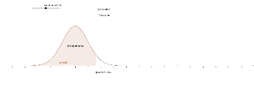
①This GeoGebra example dynamically illustrates the construction and visualization of confidence intervals for a normal distribution, showing the probabilistic relationship between sample statistics and population parameters. ②Core mathematical concepts include confidence intervals, normal distribution, significance level, critical values, and probability area via integration, with symmetry, arithmetic operations, and trigonometric functions used for auxiliary plotting. ③Construction details: The InverseNormal command computes normal quantiles (e.g., z-scores), and the Integral command calculates the probability area under the curve; objects include the normal density function (stfrv), interval boundaries (Öryggismörk, Neðrimörk), auxiliary points (a,b,c,d,e,g,h), and text labels (texti1,texti2,texti3), with sliders or parameters to adjust the confidence level. ④Suitable for high school and introductory university statistics courses, helping students understand the meaning of confidence intervals, the trade-off between confidence level and interval width, and practical applications of normal distribution probability calculations.