
Complex Linear Mapping Diagrams I (Circles)
Loading the math board and drawing, please wait…
In collections
Mapping Diagrams to Visualize Complex Analysis
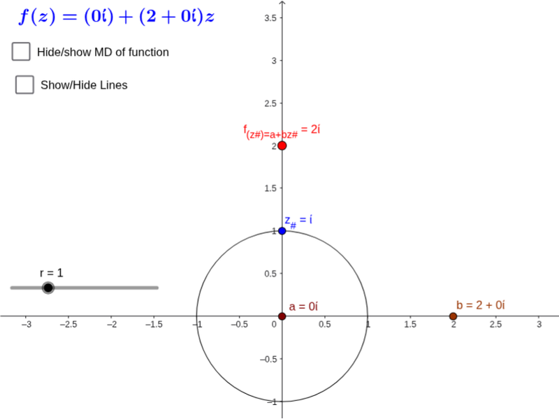
This example demonstrates how circles transform under complex linear mappings. Key mathematical concepts include complex numbers, linear mappings, and properties of circles. Using GeoGebra commands such as Sequence, CurveCartesian, and Vector, the example dynamically shows the effect of complex linear mappings on circles. Suitable for high school mathematics education and learning.
GeoGebra Commands & Parameters
Sequence((r * (cos(t) + (sin(t) * ί))), t, -3.141592653589793, 3.141592653589793, 0.5235987755982988) → z_*Sequence((x(Element[fz_*, k]), y(Element[fz_*, k]), height_{image}), k, 1, 12) → fpoint_*Sequence(Vector[Element[z_*, j], Element[fpoint_*, j]], j, 1, 12) → fvec_*CurveCartesian((r * cos(t)), (r * sin(t)), height_{image}, t, 0, 6.283185307179586) → dVector(z_#, f_{(z#)=a+bz#.}) → wCurveCartesian(t, 0, height_{image}, t, -5, 5) → XhCurveCartesian(0, t, height_{image}, t, -5, 5) → YhSequence(Line[Element[z_*, j], Element[fpoint_*, j]], j, 1, 12) → fline_*Textfield(F) → inputBox1Point(c) → ALocus(PF_A, A) → loc1
AI Drawing Prompt Reference
Draw a circle and apply a linear mapping transformation to observe how the circle changes. First, create a circle with radius r, then generate a series of points on the circle using parameter t from -π to π. Next, apply a linear mapping to these points to form a new sequence of points. Connect these new points to form a new curve. Finally, adjust parameters a and b to observe the changes in the circle under different linear mappings.
The prompt above was compiled from the original drawing commands and is for reference only.