
Complex Integration: z^2 over line segment
Loading the math board and drawing, please wait…
In collections
Mapping Diagrams to Visualize Complex Analysis
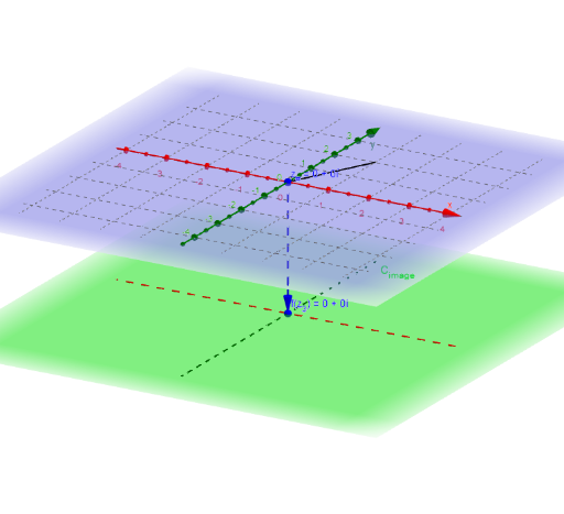
This example demonstrates the computation of the integral of z^2 along a line segment in the complex plane. Key math concepts include complex numbers, integration, and line segment parametrization. GeoGebra commands and objects like Sequence, Zip, Vector, CurveCartesian, Sphere, Intersect, Segment, and Textfield are used to construct the integration path and visualize the result, making it suitable for high school and above students learning complex integration techniques and geometric interpretations.
GeoGebra Commands & Parameters
Sequence(t, t, t_0 + dt, t_1 + dt, dt) → t_3Zip(x_C(B) + (y_C(B) * ί), B, t_3) → z_1Sequence(t, t, t_0, t_1, dt) → t_*Zip(x_C(B) + (y_C(B) * ί), B, t_*) → z_*Zip(t - u, t, z_1, u, z_*) → dz_*Sequence((Element[fz_*, k] * Element[dz_*, k]), k, 1, n) → fdz_*Sequence(Sum[fdz_*, k], k, 1, n) → SUMfdz_*Zip((x(B), y(B), ht), B, fz_*) → fpoint_*Vector(z_#, f_{(z#).}) → wCurveCartesian(t, 0, ht, t, -5, 5) → XhCurveCartesian(0, t, ht, t, -5, 5) → YhSphere((0, 0, 4), 1) → RSIntersect(zAxis, RS, 2) → ASegment(A, f_{(z#).}) → f_sIntersect(f_s, RS) → P_∞, CZip((x(Z), y(Z), ht), Z, SUMfdz_*) → ESumSequence(Element[dz_*, k], k, 1, n) → dz_nCurveCartesian(x_C(t), y_C(t), t, t_0, t_1) → cTextfield(x_C) → inputBox4Textfield(y_C) → inputBox5Vector(z_#, Pointfz_#) → uTextfield(F) → InputBox1Zip(Vector[A, B], A, z_*, B, ESum) → ESumV_*Zip(Vector[A, B], A, z_*, B, fpoint_*) → fvec_*