Complex Line Integral: Definition and F.T. Examples

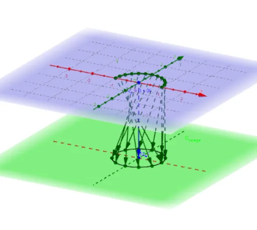
Loading the math board and drawing, please wait…

2017-12-31 06:22

In collections Mapping Diagrams to Visualize Complex Analysis

This example demonstrates the calculation process of complex line integrals and applications of Fourier Transform. It involves core mathematical concepts like complex numbers, integration, parametric equations, and coordinate geometry. GeoGebra commands and objects used include Element, Sequence, Zip, If, CurveCartesian, Textfield, Vector, Integral, Point, Locus. Suitable for university mathematics students or those studying complex functions and integrals.

GeoGebra Commands & Parameters

Element(zfnlist, n_f) → F
Element(yfnlist, n_γ) → y_γ
Element(xfnlist, n_γ) → x_γ
Sequence(t, t, t_0 + dt, t_2 + dt, dt) → t_1
Zip(x_γ(B) + (y_γ(B) * ί) + z_#, B, t_1) → z_1
Sequence(t, t, t_0, t_2, dt) → t_*
Zip(x_γ(B) + (y_γ(B) * ί) + z_#, B, t_*) → z_*
Zip(t - u, t, z_1, u, z_*) → dz_*
If(Align ≟ 1, z_# - fz_#, 0) → align
Sequence(((Element[fz_*, k] - align) * Element[dz_*, k]), k, 1, n) → fdz_*
Sequence(Sum[fdz_*, k], k, 1, n) → SUMfdz_*
Zip((x(B), y(B), ht), B, fz_*) → fpoint_*
Zip((x(Z) + x(align), y(Z) + y(align), ht), Z, SUMfdz_*) → ESum
Sequence(Element[dz_*, k], k, 1, n) → dz_n
CurveCartesian(x_γ(t) + x(z_#), y_γ(t) + y(z_#), t, t_0, t_2) → γ
Textfield(x_γ) → inputxt
Textfield(y_γ) → inputyt
Vector(z_#, Pfz_#) → u
Textfield(F) → InputFz
Zip(Vector[A, B], A, z_*, B, fpoint_*) → fvec_*
Integral(f) → Int_f
Element(z_*, 1) → z_0
Element(z_*, n + 1) → z_2
Point(γ) → Aγ
Locus(FAγ3, Aγ) → fLoc
Zip(Vector[A, B], A, z_*, B, ESum) → ESumV_*
CurveCartesian(t + x(align), y(align), ht, t, -5, 5) → Xh
CurveCartesian(x(align), t + y(align), ht, t, -5, 5) → Yh