
Complex Integration: z^2 over Curve
Loading the math board and drawing, please wait…
In collections
Mapping Diagrams to Visualize Complex Analysis
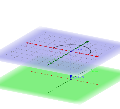
This example demonstrates the complex integration of z^2 over a curve. Key mathematical concepts include complex integration and parametric curves. Using GeoGebra commands such as Sequence, Zip, Vector, and CurveCartesian, the path of integration and the changing integral values are visually illustrated. Suitable for university-level complex function studies.
GeoGebra Commands & Parameters
Sequence(t, t, t_0 + dt, t_1 + dt, dt) → t_3Zip(x_C(B) + (y_C(B) * ί), B, t_3) → z_1Sequence(t, t, t_0, t_1, dt) → t_*Zip(x_C(B) + (y_C(B) * ί), B, t_*) → z_*Zip(t - u, t, z_1, u, z_*) → dz_*Sequence((Element[fz_*, k] * Element[dz_*, k]), k, 1, n) → fdz_*Sequence(Sum[fdz_*, k], k, 1, n) → SUMfdz_*Zip((x(B), y(B), ht), B, fz_*) → fpoint_*Vector(z_#, f_{(z#).}) → wCurveCartesian(t, 0, ht, t, -5, 5) → XhCurveCartesian(0, t, ht, t, -5, 5) → YhSphere((0, 0, 4), 1) → RSIntersect(zAxis, RS, 2) → ASegment(A, f_{(z#).}) → f_sIntersect(f_s, RS) → P_∞, CZip((x(Z), y(Z), ht), Z, SUMfdz_*) → ESumSequence(Element[dz_*, k], k, 1, n) → dz_nCurveCartesian(x_C(t), y_C(t), t, t_0, t_1) → cTextfield(x_C) → inputBox4Textfield(y_C) → inputBox5Vector(z_#, Pointfz_#) → uTextfield(F) → InputBox1Zip(Vector[A, B], A, z_*, B, ESum) → ESumV_*Zip(Vector[A, B], A, z_*, B, fpoint_*) → fvec_*
AI Drawing Prompt Reference
Draw the integral path of the complex curve z^2 from t_0 to t_1. First, draw the parametric curve c, then calculate z_1 and z_*, followed by dz_* and fdz_*, and finally calculate SUMfdz_*. Also, plot the integral path on the z-axis to show the change in integral values.
The prompt above was compiled from the original drawing commands and is for reference only.