
Completing the Square for Quadratic Equation (II) : Solving the Equation
Loading the math board and drawing, please wait…
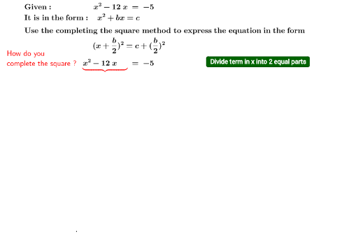
This example demonstrates how to solve quadratic equations using the method of completing the square, involving core mathematical concepts such as completing the square and solving quadratic equations. Construction highlights extracted from the 'Construction Summary' using GeoGebra commands/objects: Point, Midpoint, RandomElement, Vector, Random, Simplify, Intersect, Polygon, Dilate, Translate, Root; objects: n_{motion}, P_{xsquared}, h, D, B, M_{BD}, a, u_1, c, b, sl1, a2, b2, sl2, sr2, s3, s4, as, bs, sl5, sr5, sl6, d, f, button1, j, m, k, l, r, e, textInstructionSlider1, textFinalText, p, q, g, i, u, t, s. Suitable for high school mathematics teaching, helping students understand and master the steps and methods of solving quadratic equations using the completing square method.
GeoGebra Commands & Parameters
Point(yAxis) → DPoint(xAxis) → BMidpoint(B, D) → M_{BD}RandomElement({-7, -6, -5, -4, -3, -2, -1, 7, 6, 5, 4, 3, 2, 1}) → aVector(P_{xsquared}, M_{BD}) → u_1Random(-7, 7) → bSimplify((x - a)^(2) - c^(2)) → sl1Simplify(y^(2) + (b2 * y)) → sr2Simplify((-((x - a)^(2) - c^(2) - x^(2) - (a2 * x)))) → s3Simplify(x^(2) + (a2 * x)) → s4Simplify((x - a)^(2)) → sl5Simplify((y - b)^(2)) → sr5Simplify(x - h) → sl6Intersect(xAxis, yAxis) → APolygon(A, B, C, D) → poly1, a_1, b_1, c_1, d_1Point(xAxis) → EPoint(xAxis) → FPolygon(E, F, G, H) → poly2, e_1, f_1, g_1, h_1Polygon(I, J, K, L) → poly3, i_1, j_1, k_1, l_1Polygon(M, N, O, P) → poly4, m_1, n_1, o_1, p_1Dilate(M, h / a, O) → M'Dilate(N, h / a, O) → N'Dilate(O, h / a, O) → O'Dilate(P, h / a, O) → P'Polygon(M', N', O', P') → poly4', m', n', o', p'Midpoint(A, B) → M_{AB}Midpoint(A, D) → M_{AD}Midpoint(E, F) → M_{EF}Midpoint(F, H) → M_{FH}Midpoint(I, L) → M_{IL}Midpoint(J, L) → M_{JL}Midpoint(N', P') → M_{NP}Translate(P_{xsquared}, Vector[(n_{motion} * u_1)]) → RVector(P_{xsquared}, R) → v_1Vector(P_{bx}, M_{FH}) → u_2Translate(P_{bx}, Vector[(n_{motion} * u_2)]) → QVector(P_{bx}, M_{JL}) → u_3Translate(P_{bx}, Vector[(n_{motion} * u_3)]) → SVector(P_{bx}, Q) → v_2Vector(P_{bx}, S) → v_3Dilate(M, j / a^(2), O) → M'_1Dilate(N, j / a^(2), O) → N'_1Dilate(O, j / a^(2), O) → O'_1Dilate(P, j / a^(2), O) → P'_1Polygon(M'_1, N'_1, O'_1, P'_1) → poly4'_1, m'_1, n'_1, o'_1, p'_1Random((-(a2 / 2)^(2)) + 1, 8) → c_RRoot(x^(2) + (a2 * x) - c_R) → T_{1st of roots}, U_{2nd of roots}
AI Drawing Prompt Reference
Draw a quadratic equation graph and solve it using the completing the square method. Start by creating points D and B on the coordinate axes, then randomly generate values for a and b. Construct the quadratic equation graph with translations and scaling transformations, and finally obtain the two roots T_{1st of roots} and U_{2nd of roots}.
The prompt above was compiled from the original drawing commands and is for reference only.