
CIS.PSMPDI Scalar Multiple Property 'Proof'
Loading the math board and drawing, please wait…
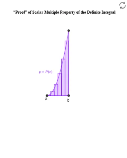
① This GeoGebra example dynamically demonstrates a geometric 'proof' of the Scalar Multiple Property, typically illustrating the linear relationship under scalar multiplication for vectors or functions. ② Core mathematical concepts include vector operations, scalar multiplication, function graphs, and the relationship between integrals and areas, possibly also involving arithmetic mean and quadratic equations. ③ Construction highlights: from the summary, commands such as Integral and RectangleSum are used to build area approximations; basic objects like Point, Line, Vector, Segment construct the geometry; Sequence, Zip, and TableText generate data tables; Textfield and input boxes enable interactive parameter adjustment. Objects include multiple points, axes, functions, and text labels. ④ Suitable for high school to early college students, this helps understand the geometric impact of scalar multiplication on functions or vectors, and serves as an intuitive teaching tool for the linearity property of integrals in calculus.
GeoGebra Commands & Parameters
Integral(P, a, c) → IPacIntegral(P, c, b) → IPcbIntegral(P, a, b) → IPabTextfield(P) → inputBox1Point(yAxis) → DPoint(yAxis) → ELine(D, E) → XaxisLine(Ypt, Xaxis) → YaxisVector(G, J) → uVector(I, F) → vVector(H, K) → wSegment(F, K) → fSegment(F, J) → hSegment(I, H) → iSegment(G, I) → jIntegral(αP, a, b) → IαPabLine(M, Yaxis) → Y2axisVector(J, αs_a) → eVector(K, αs_b) → dSegment(αs_a, αs_b) → gSegment(J, K) → mSegment(G, H) → pTextfield(Q) → InputBox1Integral(Q, a, b) → IQabIntegral(P(x) + Q(x), a, b) → IPQabLine(O, Xaxis) → qVector(G, SQa) → rVector(H, SQb) → sSegment(SQb, SQa) → tVector(K, SPQb) → u_1Vector(SQb, SPQb) → v_1Vector(SQa, SPQa) → w_1Segment(SPQb, SPQa) → f_1Vector(SQb, SQb1) → a_1Segment(SPQb, SQb1) → g_1Segment(SQb1, SPQa) → h_1Vector(J, SQb1) → b_1Point(f_1) → RSequence(1, n) → NZip((0, a + (k * dx)), k, N) → x_1Zip(a - dx / 2 + (k * dx), k, N) → c_*Zip(Sum[Pcdx_*, k], k, N) → SPcdx_*Zip(Sum[αPxdx_*, k], k, N) → SαPcdx_*Zip((x(Ypt), sp), sp, SPcdx_*) → SptPcdx_*Zip(Vector[A, B], A, x_1, B, SptPcdx_*) → vecSP_*Zip((x(M), sp), sp, SαPcdx_*) → SptαPcdx_*Zip(Vector[A, B], A, SptPcdx_*, B, SptαPcdx_*) → vecSαP_*TableText(Transpose[{Join[{{"c_k"}, c_*}], Join[{{"P(c_k)Δx"}, Pcdx_*}], Join[{{"αP(c_k)Δx"}, αPxdx_*}]}], "|_cc") → TableIRectangleSum(P, y(G), y(H), n, 1 / 2) → GrMidEstIntPRectangleSum((α * P(x)), y(G), y(H), n, 1 / 2) → GrMidestIntαP
AI Drawing Prompt Reference
Draw a dynamic geometric proof of the scalar multiple property, showing vector operations, function graphs, and the relationship between integrals and areas. Include basic geometric objects like points, lines, vectors, and segments, with integral and rectangle sum constructions for area approximations. Use sliders for interactive parameter adjustment, generate data tables with labels, and illustrate the geometric impact of scalar multiplication on functions or vectors, as well as the linearity property of integrals in calculus.
The prompt above was compiled from the original drawing commands and is for reference only.