
Center and Spread Problems
Loading the math board and drawing, please wait…
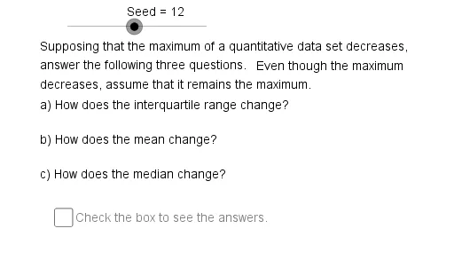
This example illustrates the concepts of center and spread, including mean and standard deviation. Using GeoGebra commands like Sequence and Element, it dynamically shows the central tendency and dispersion of a dataset. Suitable for statistics and probability studies.
GeoGebra Commands & Parameters
Sequence(Mod[8 + (23 * k), 48] + 100, k, 0, 47) → ChNmSqElement(ChNmSq, Seed) → ChNm1Mod(ChNm2, 2) → Op2Mod(ChNm1, 2) → Op1If(Op1 ≟ 0, "minimum", "maximum") → MnOrMxIf(Op2 ≟ 0, "decreases", "increases") → DnOrUpIf(Op1 ≟ 0, If[Op2 ≟ 0, "increases", "decreases"], If[Op2 ≟ 0, "decreases", "increases"]) → SpDrMod(ChNm3, 6) → Op3Sequence(Mod[Str + k, 6] + 1, k, 1, 3) → ObChSqText("mean") → Ob1Text("median") → Ob2Text("midrange") → Ob3Text("range") → Ob4Text("standard deviation") → Ob5Text("interquartile range") → Ob6Element(ObSq, Element[ObChSq, 1]) → ObAElement(ObSq, Element[ObChSq, 2]) → ObBElement(ObSq, Element[ObChSq, 3]) → ObCElement(AnSq, Element[ObChSq, 1]) → ChAElement(AnSq, Element[ObChSq, 2]) → ChBElement(AnSq, Element[ObChSq, 3]) → ChC