
CCGPS CA 4.2.2 Example 2: Modeling Student Enrollment with Exponential Functions
Loading the math board and drawing, please wait…
In collections
CCGPS CA Unit 4 Lesson 2
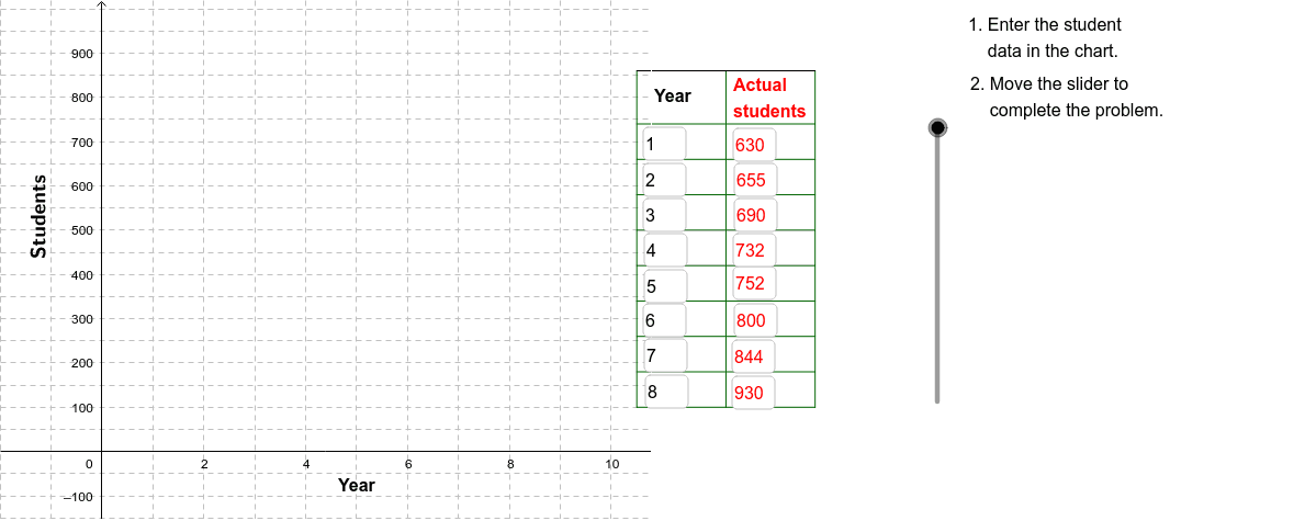
Example 2 of CCGPS CA 4.2.2 illustrates how to use GeoGebra to create a scatter plot of eight years of student enrollment data and fit an exponential function to model the growth trend. The construction employs Corner, Textfield, Sequence, Segment, Polygon, and VerticalText commands, generating objects such as A1–B9 and a Slid slider for parameter adjustment. Core concepts include exponential functions, regression analysis, scatter plots, means, distributions, and linear programming optimization. This resource is ideal for high‑school students studying exponential modeling and for introductory college statistics or mathematical modeling courses.
GeoGebra Commands & Parameters
Corner(2) → Corn2Corner(3) → Corn3Textfield(A2) → InA2Textfield(A3) → InA3Textfield(A4) → InA4Textfield(A5) → InA5Textfield(A6) → InA6Textfield(A7) → InA7Textfield(A8) → InA8Textfield(A9) → InA9Textfield(B9) → InB9Textfield(B8) → InB8Textfield(B7) → InB7Textfield(B6) → InB6Textfield(B5) → InB5Textfield(B4) → InB4Textfield(B3) → InB3Textfield(B2) → InB2Sequence(Segment[(10.5, 100 + (80 * j)), (14, 100 + (80 * j))], j, 0, 8) → LnListSequence(Segment[(14, 100 + (80 * j)), (16, 100 + (80 * j))], j, 0, 8) → LnList3Sequence(Segment[(10.5 + (1.75 * j), 100), (10.5 + (1.75 * j), 860)], j, 0, 2) → LnList2Segment((10.5, 860), (14, 860)) → Top1Segment((14, 860), (16, 860)) → Top2Segment((16, 100), (16, 860)) → Side1Polygon((0.5 * Corner[1]) + (0.5 * Corner[2]), Corner[2], Corner[3], (0.5 * Corner[3]) + (0.5 * Corner[4])) → poly1, b, c, d, eVerticalText("Students") → Students
AI Drawing Prompt Reference
Create a scatter plot of eight years of student enrollment data with an exponential fit. Draw a grid: horizontal lines from y=100 to 860 every 80 units, vertical lines from x=10.5 to 14 every 1.75 units, plus top and right border segments; fill the background with a rectangle covering half the view. Place a vertical “Students” label on the left. Provide eight editable text boxes for the years (A2‑A9) and enrollment numbers (B2‑B9), and add a slider to adjust the exponential model parameters so the fitted curve updates interactively.
The prompt above was compiled from the original drawing commands and is for reference only.