
Bugwelle Example
Loading the math board and drawing, please wait…
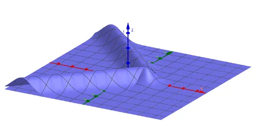
This example demonstrates the graphical representation and properties of the Bugwelle function, involving linear optimization, cubes, step functions, real numbers, and isosceles triangles. It uses GeoGebra commands like t, f_1, f_2, f_3 for function definition and dynamic visualization, suitable for high school and above mathematics education focusing on function analysis and geometric transformations.
GeoGebra Commands & Parameters
Numeric t(1.25)f_1(x, y) = If[x < t, ℯ^((-(x + y - t)^(2)))]f_2(x, y) = If[x < t, ℯ^((-(x - y - t)^(2)))]f_3(x, y) = ℯ^((-2 * ((x - t)^(2) + y^(2))))
AI Drawing Prompt Reference
Create a dynamic visualization showing the graph of a function composed of three parts: when x is less than a slider t, the first part is the negative exponential of the square of x+y-t, the second part is the negative exponential of the square of x-y-t, and the third part is the negative exponential of twice the square of x-t plus y squared. Include a cube and an isosceles triangle, highlighting the optimization process and the stepwise changes in the function.
The prompt above was compiled from the original drawing commands and is for reference only.