
Boxplot Construction Example
Loading the math board and drawing, please wait…
In collections
Numeracy Practice
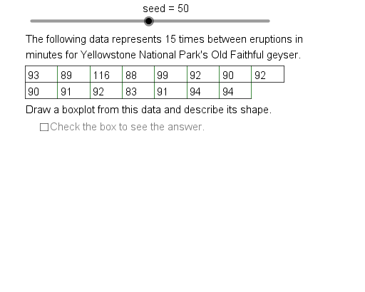
This example demonstrates how to construct a boxplot using GeoGebra, visually representing data distribution characteristics. Key mathematical concepts involved include statistical measures such as median, quartiles, and range, along with data sorting and interval partitioning. The construction leverages GeoGebra commands/objects like Element, Sequence, Min, Max, If, Q3, Q1, Sort, Median, Intersection, CountIf, KeepIf, Segment, Midpoint, Union, and objects including seed, PrmFct, Cmpst, Nmbr1 to Nmbr4, Chc4 to Chc1, Size, DD5 to DD1, Unt5 to Unt1, Ttl5 to Ttl1, Strt, Rate, OpSq, DS1 to DS5, DSSq, DataSet, DS0. It is suitable for high school mathematics courses in statistics and probability, serving as a teaching demonstration or for student exploratory learning.
GeoGebra Commands & Parameters
Element(RPSq, Chc3) → RateSequence(Mod[Strt + (Rate * k), 23] + 1, k, 0, 22, 1) → OpSqElement(DSSq, DataSet) → DS0Sequence(Element[DS0, Element[OpSq, k]], k, 1, Size) → SampleMin(Sample) → OldMnMax(Sample) → OldMxIf((5 * AxUntLB) ≤ AxUntUB, (5 * AxUntLB), If[(2 * AxUntLB) ≤ AxUntUB, (2 * AxUntLB), AxUntLB]) → AxUntElement(AcSq, DataSet) → AccQ3(Sample) → SmpQ3Q1(Sample) → SmpQ1Sequence(k, k, OldMn, OldMx, Acc) → DomainSort(Intersection[Domain, Sample]) → RangeMedian(Sample) → SmpMdnSequence(k, k, (ceil(LoFn / Acc) * Acc), (floor(UpFn / Acc) * Acc), Acc) → MiddleIntersection(Sample, Middle) → GoodDataMin(GoodData) → NwMnCountIf(x < LoFn, Range) → LfOtlrCntRngMax(GoodData) → NwMxCountIf(x > UpFn, Range) → RtOtlrCntRngKeepIf(x > UpFn, Range) → DmAbFnCountIf(x ≤ OldMx, Range) → RngCntSegment(AxLE, AxRE) → axisSegment(NMinT, NMinB) → nwminMidpoint(nwmin) → NMinMSegment(QLoT, QLoB) → qloSegment(MedT, MedB) → medMidpoint(qlo) → QLoMSegment(NMinM, QLoM) → lfwhSegment(QHiT, QHiB) → qhiSegment(QLoT, QHiT) → boxtopSegment(QLoB, QHiB) → boxbotSegment(NMaxT, NMaxB) → nwmaxMidpoint(nwmax) → NMaxMMidpoint(qhi) → QHiMSegment(QHiM, NMaxM) → rtwhKeepIf(x < LoFn, Range) → LfOtlrVlsCountIf(x > UpFn, Sample) → RtOtlrCntCountIf(x < LoFn, Sample) → LfOtlrCntKeepIf(x < LoFn, Range) → DmBlFnElement(DDSq, DataSet) → DD0Segment(TbUL, TbUR) → tbtpSegment(TbML, TbMR) → tbmdSegment(TbLL, TbLR) → tbbtSegment(TbUL, TbLL) → tblfSegment(TbUR, TbMR) → tbrtSequence(Segment[(TbLf + (k * TbCW), TbTp), (TbLf + (k * TbCW), TbTp - (2 * TbCH))], k, 1, DtRL2) → TbDLSqSequence(Text[k, (adp(k) - 1, AxHt - 0.07)], k, AxMn, AxMx, AxUnt) → AxLbSqSequence(Segment[(adp(k), AxHt + 0.01), (adp(k), AxHt - 0.01)], k, AxMn, AxMx, AxUnt) → AxTcSqSequence((adp(Element[DmAbFn, k]), AxHt + 0.2), k, 1, RtOtlrCntRng) → RtOtlrSequence((adp(Element[LfOtlrVls, k]), AxHt + 0.2), k, 1, LfOtlrCntRng) → LfOtlrSqKeepIf(x > UpFn, Range) → RtOtlrVlsUnion(RtOtlrVls, LfOtlrVls) → OutliersElement(UntSq, DataSet) → Unt0Element(TtlSq, DataSet) → Ttl0If(WhLnRt > WhLnLf + (0.05 * ScFc), 1, If[WhLnLf > WhLnRt + (0.05 * ScFc), 2, If[BxLnRt > BxLnLf + (0.05 * ScFc), 3, If[BxLnLf > BxLnRt + (0.05 * ScFc), 4, 5]]]) → ShpNmbSequence(Text[Element[Sample, k + DtRL1], (TbLf - 5.5 + (k * 6), TbTp - TbCH - 0.08)], k, 1, DtRL2) → DRw2Sequence(Text[Element[Sample, k], (TbLf - 5.5 + (k * 6), TbTp - 0.08)], k, 1, DtRL1) → DRw1
AI Drawing Prompt Reference
Create a boxplot to visually represent data distribution characteristics, highlighting statistical measures like median, quartiles, and range. Identify the minimum and maximum values in the dataset, then determine the first quartile (Q1) and third quartile (Q3). Draw the box on the axis between Q1 and Q3, with a line inside representing the median. Extend whiskers from the box to the minimum and maximum values. Label the axis with appropriate intervals.
The prompt above was compiled from the original drawing commands and is for reference only.