
Biscribed Orthotruncated Propello Icosahedron (V=120) and Its Dual: Edge/Face Co
Loading the math board and drawing, please wait…
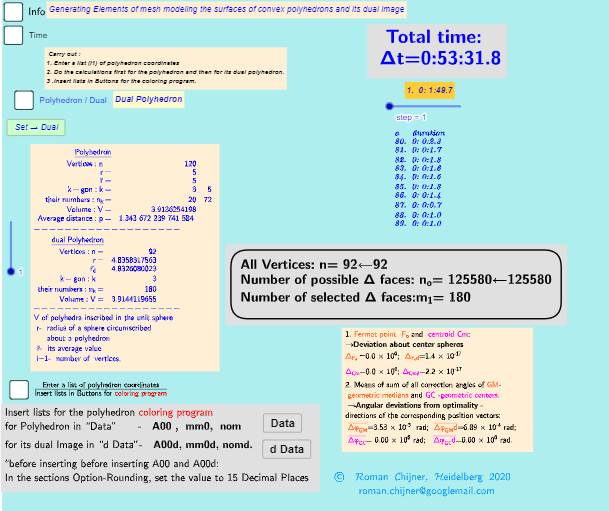
This example visualizes the Biscribed Orthotruncated Propello Icosahedron with volume parameter V=120 and its dual polyhedron image, using systematic coloring of both edges and faces to reveal the correspondence and symmetry between the primal and dual structures. Key mathematics includes solid geometry of an orthotruncated propello icosahedron, the duality relationship between polyhedra (face–edge/vertex correspondence), and measurement-driven computation involving volume-related quantities (e.g., constructing or comparing spherical/enclosing volume parameters and related radii/derived values). Construction details in GeoGebra rely on label and data presentation via Text and TableText; object selection and mapping via If, IndexOf, Element, and Sequence; and numerical aggregation/control using Sum, Max, Length, and Div. The model organizes geometric/metric variables such as r_m, Volsphere, Vol, Vol_r, A00/A00d, and r_d, and provides interactive control elements (e.g., button3 and index variables) to switch or drive the coloring and dual-image generation. Suitable for high school to early university levels for teaching/learning polyhedral duality and geometric construction through an interactive, color-coded representation.
GeoGebra Commands & Parameters
Text("" + p) → txt_pSum(Flatten[Sequence[Append[Sequence[Element[txt_p, i], i, m01(k), m02(k)], " "], k, 1, 5]]) → txtUm1If(bu0, A00, A00d) → A00_0Length(A00_0) → nLength(l2) → läl2Sequence(sgn(Determinant[{Element[A00_0, i1] - Element[A00_0, j], Element[A00_0, i2] - Element[A00_0, j], Element[A00_0, i3] - Element[A00_0, j]}]), j, 1, n) → l01Length(A00d) → zzzSum(Zip[(T * F), T, SysTimeAkt1, F, {1, 1000, 60000, 3600000, 86400000}]) → TimeAbs1Sum(Zip[(T * F), T, SysTimeAkt2, F, {1, 1000, 60000, 3600000, 86400000}]) → TimeAbs2Div(TimeRelab, 3600) → HDiv(TimeRelab - (H * 3600), 60) → MElement(ZwZeit, step) → text10TableText({Append["a duration", Last[ZwZeit, Min[10, Length[ZwZeit]]]]}, "v") → text2cLength(A00) → lm1If(Length[Unique[l01 \ {0}]] ≟ 1, 7, -7) → a7Sum(Zip[(T * F), T, SysTimeAkt0, F, {1, 1000, 60000, 3600000, 86400000}]) → TimeAbs0Div(TimeRelab0, 3600) → H0Div(TimeRelab0 - (H0 * 3600), 60) → M0Text("" + (TimeRelab0 - (H0 * 3600) - (M0 * 60))) → S0aText("" + (TimeRelab - (H * 3600) - (M * 60))) → SIndexOf(".", S) → indexIndexOf(".", S0a) → indexaFirst(S, index + 1) → txtSFirst(S0a, indexa + 1) → txtS0aIf(bu0, " ", "d") → txtbuoMax(Length[A00], Length[A00d]) → maxläElement(A00, 24) → m11TableText({{"\underline{Polyhedron}"}, Append["Vertices: n=", {Length[A00]}], Append["r=", {r}], Append["\bar{r}=", {r_m}], Append["k-gon : k=", mm5a], Append["their\; numbers: n_k=", mm7a], Append["Volume: V=", {Vol_r}], Append["Average\; distance: p=", {txtUm1}]}, "hr ") → text7TableText({{"\underline{dual\;Polyhedron}"}, Append["Vertices: n=", {Length[A00d]}], Append["r=", {r_d}], Append[" \bar{r_d}= ", {r_md}], Append["k-gon : k=", mm5ad], Append["their\; numbers: n_k=", mm7ad], Append["Volume: V=", {Vold_r}]}, "hr ") → text20
AI Drawing Prompt Reference
Visualize a 'Biscribed Orthotruncated Propello Icosahedron' polyhedron with 120 vertices and its dual polyhedron. Use systematic edge and face coloring to highlight the correspondence and symmetry between the two structures. Display key parameters like volume, average distance, and vertex counts for both polyhedra, emphasizing their dual relationships. Clearly label and color-code each polyhedron's features to illustrate geometric relationships and symmetry.
The prompt above was compiled from the original drawing commands and is for reference only.