
Binomial Distribution Demo by loreang98
Loading the math board and drawing, please wait…
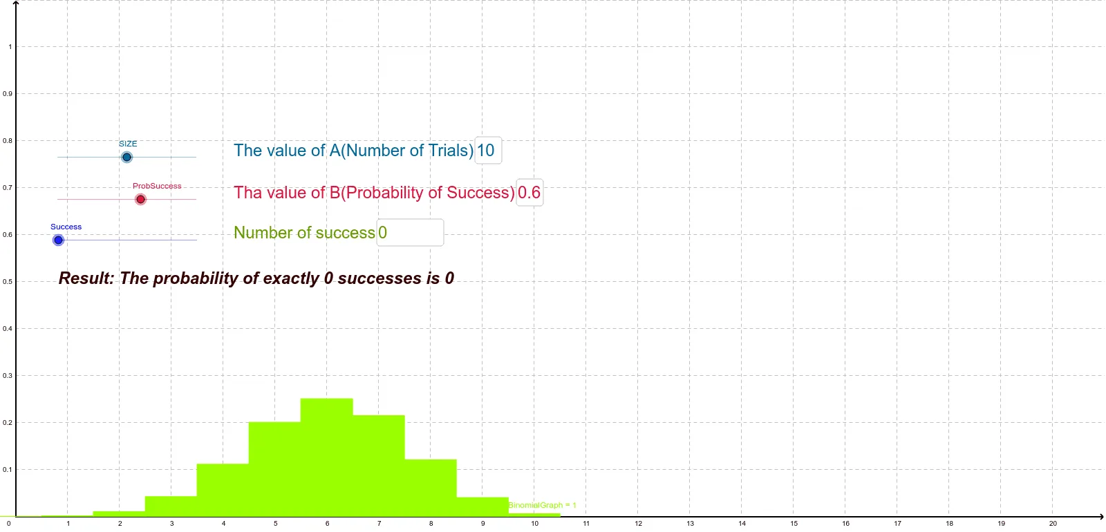
This example demonstrates the binomial distribution's probability distribution graph and statistical characteristics. Key math concepts include binomial distribution, arithmetic mean, probability, exponent, and statistical properties. Construction highlights involve using GeoGebra commands like BinomialDist for graphing, combined with Textfield, Sequence, Element to showcase distribution features. Interactive parameter adjustments are made via inputBoxes (inputBox1, inputBox2, inputBox3), with Fix_x, Fix_y defining axes, Success calculating success probability, ResultList storing outcomes, and Probability displaying probability values. Suitable for high school and above learners to understand binomial distribution in probability statistics and its applications.
GeoGebra Commands & Parameters
BinomialDist(SIZE, ProbSuccess) → BinomialGraphTextfield(SIZE) → inputBox1Textfield(ProbSuccess) → inputBox2Textfield(Success) → inputBox3Sequence(((Binomial[SIZE, E] * ProbSuccess^(E)) * (1 - ProbSuccess)^(SIZE - E)), E, 0, SIZE) → ResultListElement(ResultList, Success + 1) → Probability
AI Drawing Prompt Reference
Draw a probability distribution graph of the binomial distribution. The graph shows the probability of success p and the number of trials n. The x-axis represents the number of successes, and the y-axis represents the probability. Include a histogram showing the probability values for different numbers of successes. Add text boxes to display key parameters like the success probability and number of trials. The graph should clearly show the statistical features of the binomial distribution, suitable for learning probability and statistics.
The prompt above was compiled from the original drawing commands and is for reference only.