
Bifurcation Diagram of Logistic Map
Loading the math board and drawing, please wait…
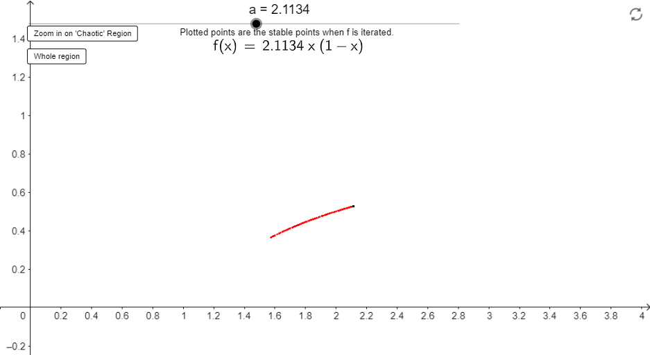
This example demonstrates the bifurcation diagram of the Logistic Map, showcasing how stable points evolve with varying parameters, a key phenomenon in chaos theory. Core math concepts include limits, iterative functions, stability analysis, and stochastic processes. GeoGebra commands used are Max, Min, and LaTeX, with objects like parameters a, function f, and auxiliary points A1-A35. Suitable for high school students and math enthusiasts interested in chaos theory.
GeoGebra Commands & Parameters
Max(x(Corner[1]), 0) → leftMin(4, x(Corner[3])) → rightLaTeX(f, true, true) → text1
AI Drawing Prompt Reference
Draw the bifurcation diagram of the Logistic Map to show how stable points evolve with varying parameters, illustrating key concepts in chaos theory such as limits, iterative functions, stability analysis, and stochastic processes. Include boundaries determined by coordinates and a function expression in LaTeX format.
The prompt above was compiled from the original drawing commands and is for reference only.