
Best Fit Lines Demonstration
Loading the math board and drawing, please wait…
In collections
statistics
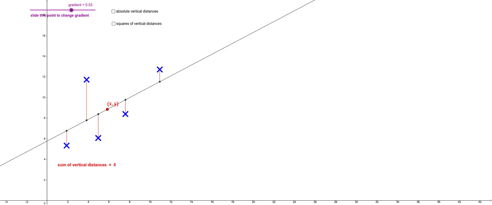
This example demonstrates how to analyze data trends by calculating and drawing best fit lines. It involves core mathematical concepts like linear regression, coordinate geometry, distance calculation, and statistical distributions. Key GeoGebra commands and objects used include OrthogonalLine, Intersect, Segment, and Midpoint. Suitable for high school students learning data fitting and statistical graphing.
GeoGebra Commands & Parameters
OrthogonalLine(E, xAxis) → eIntersect(e, g) → E'Segment(E, E') → e'OrthogonalLine(D, xAxis) → dIntersect(d, g) → D'Segment(D, D') → d'OrthogonalLine(C, xAxis) → cIntersect(c, g) → C'Segment(C, C') → c'OrthogonalLine(B, xAxis) → bIntersect(b, g) → B'Segment(B, B') → b'OrthogonalLine(A, xAxis) → aIntersect(a, g) → A'Segment(A, A') → a'Midpoint(a') → A''Midpoint(b') → B''Midpoint(c') → C''Midpoint(d') → D''Midpoint(e') → E''Segment((1, 1), (1 + squaredistancesum / 10, 1)) → fSegment((1, 2), (1 + absdistancesum / 10, 2)) → h
AI Drawing Prompt Reference
Draw a set of data points and their best fit lines. Start by drawing a vertical line from each point to the x-axis, then find the midpoints of these intersections with the x-axis. Calculate the distances from these intersections to the origin, and use these distances to draw two auxiliary lines. Finally, connect the midpoints to form the best fit lines.
The prompt above was compiled from the original drawing commands and is for reference only.