Battle Model: Differential Equation Simulation of Spartan vs Persian Forces

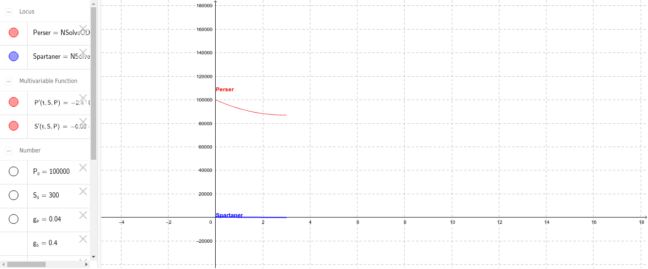
① This example uses GeoGebra's NSolveODE command to numerically solve a system of ordinary differential equations, simulating the dynamic changes in troop numbers for Spartan (S) and Persian (P) armies during a battle. ② The core mathematical concept is differential equation modeling, involving linear ODE systems, numerical solutions, parameter sensitivity analysis, and auxiliary tools like statistics and integration. ③ Construction highlights: The NSolveODE command defines derivatives S' and P', with initial values S_0 and P_0, parameters m_P, g_P, s_P controlling combat efficiency and losses, and objects Spartaner and Perser plotting troop strength over time, plus Text1 and Text2 for annotations. ④ Suitable for high school to university-level mathematical modeling courses, demonstrating numerical solutions of battle models (e.g., Lanchester equations), and useful in statistics or calculus classes to illustrate real-world applications of differential equations.