
Basic Spring Motion Model
Loading the math board and drawing, please wait…
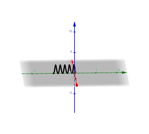
This example demonstrates the ODE model of spring motion both dampened and undampened. It involves core math concepts like differential equations, trigonometric functions, area, and centroids. Constructed using GeoGebra commands like Intersect, Segment, LaTeX, CurveCartesian, Slider Animation, and Locus. Suitable for high school and above students to understand vibration systems.
GeoGebra Commands & Parameters
Intersect(xAxis, yAxis) → BSegment(IC, B) → y'_{o}Segment(C, B) → y_{o}LaTeX(y_{D<0}, true, true) → text1LaTeX(y_{D=0}, true, true) → text2LaTeX(y_{D>0}, true, true) → text3LaTeX(D, true, true) → text4CurveCartesian(sin(((2 * pi) * s)), ((L + y_{gen}(time)) / L * s) - L, 1 - cos(((2 * pi) * s)), s, 0, L) → aCurveCartesian(sin(((2 * pi) * s)) + time, ((L + y_{gen}(time)) / L * s) - L, s, 0, L) → b
AI Drawing Prompt Reference
Draw a spring-mass system model showing the spring, mass, and support point. Use a sine function to represent the displacement of the mass. Animate the mass position at different time points using a slider. Display concepts of amplitude, period, and phase with text annotations.
The prompt above was compiled from the original drawing commands and is for reference only.