
Axial Symmetry
Loading the math board and drawing, please wait…
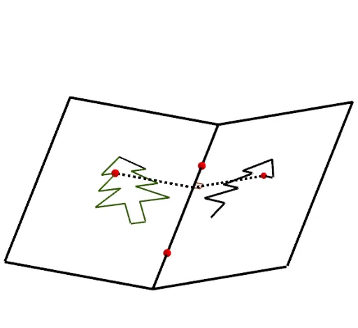
This example demonstrates the construction of axial symmetry figures. It involves key mathematical concepts such as axial symmetry and geometric construction. Using GeoGebra commands like PolyLine, Mirror, and Segment, axial symmetry figures can be constructed. Suitable for middle school and above students to learn about axial symmetry properties and geometric construction techniques.
GeoGebra Commands & Parameters
PolyLine(O_1, P_1, A_2, O_1, Q_1, R_1, S_1, T_1, U_1, V_1, W_1, Z_1) → q_1Point(q_1) → P_3PolyLine(I, H, N, M, L, K, J, I, G, F, E, D, C, B, A, O) → tPoint(t) → P1Polygon(W, Z, C_1, D_1, E_1, F_1, A_1, B_1, V) → poly2, w, z, c_1, d_1, e_1, f_1, a_1, b_1, vPoint(v) → G_1Point(v) → H_1PolyLine(A_1, F_1, B_1, A_1, E_1, D_1, C_1, Z, W, H_1, G_1, V) → p_1Point(p_1) → P2PolyLine(B_2, C_2, L_2, M_2, B_2, D_2, E_2, F_2, G_2, H_2, I_2, J_2, K_2) → r_1Point(r_1) → P4Polygon(A, B, K, L, M, N, O, C, D, E, F, G, H, I, J) → poly1, a_2, j, k, l, m, n, o, b, c, d, e, f, g, h, iLine(Q, R) → pIf(Motif ≟ 1, P1, If[Motif ≟ 2, P2, If[Motif ≟ 3, P_3, If[Motif ≟ 4, P4, P5]]]) → PMirror(P, p) → SCircle(P, a) → qLine(P, xAxis) → rIntersect(q, r) → T, USequence(Segment[Element[Marque, i], Element[Marque, i + 1]], i, 1, Length[Marque]) → TraitMirror(Trait, p) → Trait'Polygon(H_1, I_1, J_1, G_1) → poly3, h_1, i_1, j_1, g_1Mirror(H_1, p) → K_1Mirror(I_1, p) → L_1Mirror(J_1, p) → M_1Mirror(G_1, p) → N_1Polygon(K_1, L_1, M_1, N_1) → poly3', k_1, l_1, m_1, n_1Segment(P, S) → sIntersect(s, p) → N_2Angle(S, N_2, R) → αCircle(N_2, 1) → s_1Intersect(s_1, p) → O_2, P_2Intersect(s_1, s) → Q_2, R_2Line(R_2, p) → t_1Line(O_2, s) → b_2Intersect(b_2, t_1) → S_2Polygon(N_2, R_2, S_2, O_2) → poly4, n_2, r_2, s_2, o_2Segment(N_2, P) → g_2Segment(N_2, S) → f_2Rotate(Trait', rr, p) → Trait''Midpoint(Q, R) → T_2Plane(U_2, Q, R) → p_2Point(p) → V_2Point(p) → W_2OrthogonalLine(V_2, p_2) → h_2OrthogonalLine(W_2, p_2) → i_2Point(h_2) → Z_2Line(Z_2, p) → j_2Mirror(Z_2, p) → A_3Intersect(i_2, j_2) → B_3Mirror(B_3, p) → C_3Polygon(V_2, A_3, C_3, W_2) → q1, v_2, a_3, c_3, w_2Polygon(V_2, Z_2, B_3, W_2) → q2, k_2, z_2, b_3, l_2Rotate(q2, rr, p) → q2'Rotate(S, rr, p) → S'Rotate(N_2, rr, p) → D_3Rotate(S, rr, p) → S'_1Segment(D_3, S'_1) → m_2
AI Drawing Prompt Reference
Draw an axial symmetry demonstration. Start with a straight line as the axis of symmetry. Construct two polygons on opposite sides of the axis, one open polyline and one closed polygon. Place a movable point on the open polyline, then draw a perpendicular from this point to the axis. Use a circle centered at the intersection of the perpendicular and the axis to construct a small square, illustrating the local symmetry operation. Mirror the edges of the closed polygon across the axis to create its reflected counterpart, and connect corresponding points with dashed segments. Mark the angle between the perpendicular and the axis. The final figure shows the mirror symmetry of the shapes about the line.
The prompt above was compiled from the original drawing commands and is for reference only.