
Area Model for Quadratic Functions
Loading the math board and drawing, please wait…
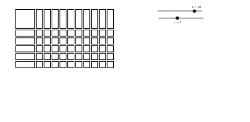
This example demonstrates how to visualize quadratic functions through a dynamic area model. It involves core math concepts like quadratic functions, area calculation, linear programming, rotation, congruence, and quadratic equations. The construction uses GeoGebra commands Polygon and Sequence, with objects such as a, A, B, C, D, poly1, a_1, e, d, c, list1, b, list2, list3, ab. It is suitable for high school mathematics education, aiding students in understanding the geometric meaning of quadratic functions and the geometric background of optimization problems.
GeoGebra Commands & Parameters
Polygon(A, B, D, C) → poly1, a_1, e, d, cSequence(Polygon[(3.25 + (1.25 * n), 3), (4.25 + (1.25 * n), 3), (4.25 + (1.25 * n), 0), (3.25 + (1.25 * n), 0)], n, 0, a - 1, 1) → list1Sequence(Polygon[(0, -0.25 - (1.25 * n)), (0, -1.25 - (1.25 * n)), (3, -1.25 - (1.25 * n)), (3, -0.25 - (1.25 * n))], n, 0, b - 1, 1) → list2Sequence(Sequence[Polygon[(3.25 + (1.25 * n), -0.25 - (1.25 * m)), (4.25 + (1.25 * n), -0.25 - (1.25 * m)), (4.25 + (1.25 * n), -1.25 - (1.25 * m)), (3.25 + (1.25 * n), -1.25 - (1.25 * m))], n, 0, a - 1, 1], m, 0, b - 1, 1) → list3
AI Drawing Prompt Reference
Create a dynamic area model to visualize quadratic functions, showing their geometric meaning and the background of optimization problems. Start by constructing a quadrilateral, then use sequences to generate multiple rectangles that stack and rotate, forming an area model representing the quadratic function. Adjust the number of rectangles dynamically using a slider to illustrate the composition of the function's graph and the change in area.
The prompt above was compiled from the original drawing commands and is for reference only.