
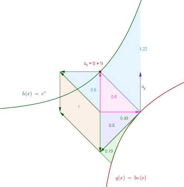
Area Diagram: Ln x vs e^x Definite Integral Visualization
Loading the math board and drawing, please wait…
In collections
Complex Math
This GeoGebra worksheet demonstrates the area under logarithmic function ln(x) and exponential function e^x, providing geometric intuition for definite integrals. Key mathematical concepts: definite integral as area under curve, inverse relationship between ln(x) and e^x, geometric meaning of integral as accumulation of area. Construction details: Polygon command for approximating curved regions; Rotate and Mirror for symmetry transformations; Intersect to find integration interval endpoints; OrthogonalLine for tangent line constructions; Textfield and InputBox for parameter interaction; Slider animation showing area accumulation. Suitable for high school calculus introduction or university-level definite integral concept visualization.
GeoGebra Commands & Parameters
Vector((a, 0)) → u_xVector((a, 0), (a, b)) → u_yVector((a, 0), (a, (2 * b))) → wVector((a, 0), (a, (3 * b))) → cPoint(u_y) → BPoint(u_y) → ASegment(B, A) → fVector((0, 0), (a, b)) → uVector((0, 0), (a, (2 * b))) → v_iRotate(u, 90*°, C) → u'Rotate(u_x, 90*°, C) → vPoint(v) → DPoint(u') → EVector(D, E) → eSegment(B, D) → iSegment(C, A) → jSegment(C, F) → kMirror(C, k) → C'Mirror(A, k) → A'Vector((a, 0), (a, b_1)) → u_1Point(u_1) → B_1Point(u_1) → A_1Segment(B_1, A_1) → f_1Textfield(a) → InputBox1Rotate(v, 180*°, C) → v'Point(v') → GVector(B, G) → mTranslate(E, v') → E'Vector(E, E') → rVector(G, E') → sPolygon(E, C, G, E') → poly1, e_1, c_1, g_2, e'Polygon(C, D, B) → poly2, b_2, c_2, d_1Polygon(C, E, D) → poly3, d_2, c_3, e_2Polygon(G, C, B_1) → poly4, b_3, g_3, c_4Intersect(h, c_2, (-5.953202266118156E-10, 0.9999999994046798)) → HIntersect(q, c_2, (1.0000000000164295, 1.642952440747795E-11)) → IPoint(h) → JPoint(h) → KPoint(h) → LPoint(h) → MPoint(h) → NPoint(h) → OPoint(h) → PPoint(h) → QPoint(h) → RPolygon(H, N, I, R, M, Q, L, O, K, P, J) → poly5, h_1, j_1, i_1, n_1, r_1, m_1, q_1, l_1, o_1, k_1, p_1Segment(B, G) → a_1OrthogonalLine(G, m) → s_1Intersect(q, s_1, (0.27846454276387034, -1.278464542751031)) → SPoint(q) → TPoint(q) → UPoint(q) → VPoint(q) → WPolygon(S, G, B, W, V, U, T) → poly6, s_2, g_4, b_4, w_1, v_1, u_2, t_1Vector((a, 0), (a, (b * 2.71))) → v_2Point(v_2) → ZPolygon(B_1, z_1, Z, N, R, M, Q, L, O, K, P) → poly7, b_5, p_2, z_3, z_2, n_2, r_2, m_2, q_2, l_2, o_2, k_2
AI Drawing Prompt Reference
Draw the graphs of ln(x) and e^x, highlighting their integral area. Use polygons to approximate curved regions, and apply rotations and reflections to show symmetry. Mark the endpoints of the integration interval and include a slider to visualize area accumulation. Add tangent lines for additional clarity, emphasizing the inverse relationship between ln(x) and e^x and the geometric interpretation of definite integrals.
The prompt above was compiled from the original drawing commands and is for reference only.